HS-1010: Simple Study Setup

In this tutorial you will learn how to setup a study on simple functions defined using a Templex template. The base input template defines two input variables, DV1 and DV2, labeled X and Y, respectively. The objective of this study is to investigate the two random variables X, Y forming the two functions X+Y and 1/X + 1/Y – 2.

This tutorial starts HyperStudy from HyperMesh Desktop > TextView. You can also start HyperStudy from HyperView, MotionView or directly in standalone mode.

The sample base input template you will use in this tutorial can be found in <hst.zip>/HS-1010/. Copy the tutorial file from this directory to your working directory.

1.	Start HyperMesh Desktop.

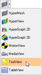
2.	On the Client Selector toolbar, select TextView.

hs_1010_01

3.	On the Standard toolbar, click .

4.	In the Open Document dialog, open the Simple.tpl file. The text editor displays the following Templex statements:

{parameter(DVAR1,"Area 1",.5,0.2,5)}

{parameter(DVAR2,"Area 2",.5,0.2,5)}

{RES = DVAR1 + DVAR2}

{CON = 1/DVAR1 + 1/DVAR2 - 2}

{RES}

{CON}

{DVAR1}

{DVAR2}

5.	On the Text toolbar, click . The text editor evaluates the Templex statements, replaces the parameters with their initial values, and displays the following results:

0.5

6.	Start HyperStudy by clicking Applications > HyperStudy from the menu bar.

1.	To start a new study, click File > New from the menu bar, or click on the toolbar.

2.	In the HyperStudy – Add dialog, enter a study name, select a location for the study, and click OK.

3.	Go to the Define Models step.

4.	Add a Parameterized File model.

a.	From the Directory, drag-and-drop the simple.tpl file into the work area.

hs_1010_drag_drop_model

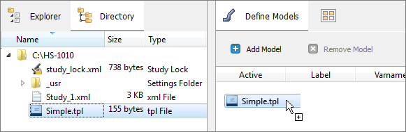
b.	In the Solver input file column, enter res. This is the name of the solver input file HyperStudy writes during the evaluation.

c.	In the Solver execution script column, select Templex (templex).

5.	Click Import Variables. Two input variables are imported from the Simple.tpl resource file.

6.	Go to the Define Input Variables step.

7.	Review the input variable's lower and upper bound ranges.

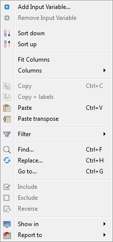
8.	Optional. Access additional editing and visualization features from the context menu by right-clicking anywhere in the work area.

hs_1010_07

9.	Go to the Specifications step.

1.	In the work area, set the Mode to Nominal Run.

2.	Click Apply.

3.	Go to the Evaluate step.

4.	Click Evaluate Tasks. An approach/nom_1/ directory is created inside the study directory. The approaches/nom_1/run__00001/m_1 directory contains the .res file, which is the result of the nominal run.

5.	Go to the Define Output Responses step.

In this step you will create two output responses.

1.	Create output response 1.

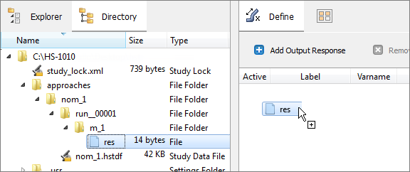
a.	From the Directory, drag-and-drop the .res file, located in approaches/nom_1/run_00001/m_1, into the work area.

hs_1010_drag_drop_res_file

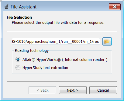
b.	In the File Assistant dialog, set the Reading technology to Altair® HyperWorks® and click Next.

hs_1010_response1_file_assist

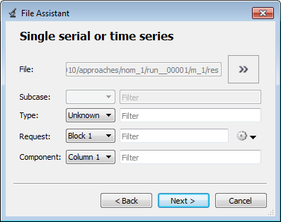
c.	Select Single item in a time series, then click Next.

d.	Define the following options, then click Next.

•	Set Type to unknown.

•	Set Request to Block 1.

•	Set Component to Column 1.

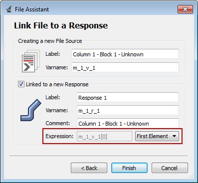
hs_1010_response1_single_serial_or_time_series

e.	Optional. Enter labels for the vector source and output response.

f.	Set Expression to First Element. The expression changes to m_1_v_1[0].

Note:

Because there is only a single value in this vector, [0] is inserted after v_1, thereby choosing the first (and only) entry in the vector.

hs_1010_15

g.	Click Finish. Output response 1 is added to the work area.

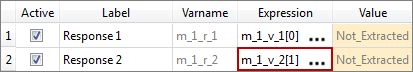
2.	Create output response 2 by repeating step 1.

3.	In the Expression field for Response 2, select the second value by changing the [0] to [1] after v_2.

hs_1010_change_expression

4.	Click Evaluate to extract the output response values.

5.	Proceed to the desired study type: DOE, Optimization, of Stochastic study.

HS-1010: Simple Study Setup

HS-1010: Simple Study Setup

HS-1010: Simple Study Setup

See Also: