HS-2215: Extensible DOE Study of a Space Frame Structure with Input Variable Constraints

In this tutorial you will use a DOE to investigate the effects of the cross sectional dimensions and joint stiffness of a truss structure’s volume and natural frequencies. The tubular truss dimensions must be constrained, such that the inner radius is always less than the outer radius. You will also use the extensible feature of the Modified Extensible Lattice Sequence in a progressive set of steps to add additional runs to a DOE.

The files used in this tutorial can be found in <hst.zip>/HS-2215/. Copy the files from this directory to your working directory.

1.	Start HyperStudy.

2.	To start a new study, click File > New from the menu bar, or click on the toolbar.

3.	In the HyperStudy – Add dialog, enter a study name, select a location for the study, and click OK.

4.	Go to the Define Models step.

5.	Add a Parameterized File model.

a.	From the Directory, drag-and-drop the tinker_toy.tpl file into the work area.

hs_2215_1

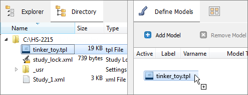
b.	In the Solver input file column, enter tinker_toy.fem. This is the name of the solver input file HyperStudy writes during any evaluation.

c.	In the Solver execution script column, select OptiStruct (os).

d.	In the Solver input arguments column, after $file, enter -core in.

This option forces OptiStruct to run with maximum memory, which will make the analysis run more quickly. The small size of the finite element model makes this possible in this example.

6.	Click Import Variables. Three input variables are imported from the tinker_toy.tpl resource file.

7.	Go to the Define Input Variables step.

8.	Review the input variable's lower and upper bound ranges.

9.	Click the Constraints tab.

10.	Add an input variable constraint.

a.	Click Add Constraint.

b.	In the Add - HyperStudy dialog, add one constraint.

c.	Define the constraint.

Note: Use the Expression Builder to select input variables to append to the Left Expression and Right Expression fields.

•	For Left Expression, enter m_1_outer_diam.

•	Set Comparison to >=.

•	For Right Expression, enter m_1_inner_diam.

11.	Go to the Specifications step.

1.	In the work area, set the Mode to Nominal Run.

2.	Click Apply.

3.	Go to the Evaluate step.

4.	Click Evaluate Tasks. An approaches/nom_1/ directory is created inside the study directory.

5.	Go to the Define Output Responses step.

1.	Create the Volume output response.

a.	From the Directory, drag-and-drop the tinker_toy.out file, located in approaches/nom_1/run_00001/m_1, into the work area.

b.	In the File Assistant dialog, set the Reading technology to Altair® HyperWorks® (HstReaderPdd) and click Next.

c.	Select Single item in a time series, then click Next.

d.	Define the following options, and then click Next.

•	Set Type to Volume.

•	Set Request to Volume.

•	Set Component to Value.

hs_2215_7

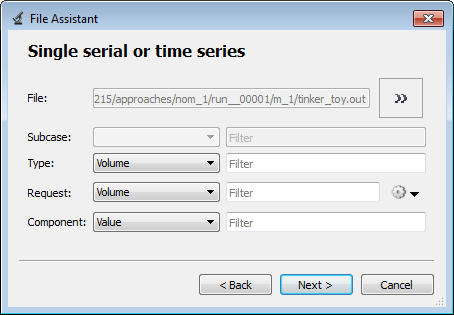
e.	Label the output response Volume.

f.	Set Expression to Maximum.

hs_2215_5

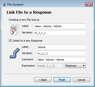
g.	Click Finish. The Volume output response is added to the work area.

2.	Create the Frequency_Vector output response, which will be used as a vector source in the frequency output responses.

a.	From the Directory, drag-and-drop the tinker_toy.out file, located in approaches/nom_1/run_00001/m_1, into the work area.

b.	In the File Assistant dialog, set the Reading technology to Altair® HyperWorks® (HstReaderPdd) and click Next.

c.	Select Multiple items at multiple time steps (readsim), then click Next.

d.	Define the following options, and then click Next.

•	Set Type to Frequency.

•	Set Request, select Mode 1 - Mode 3.

hs_2215_6

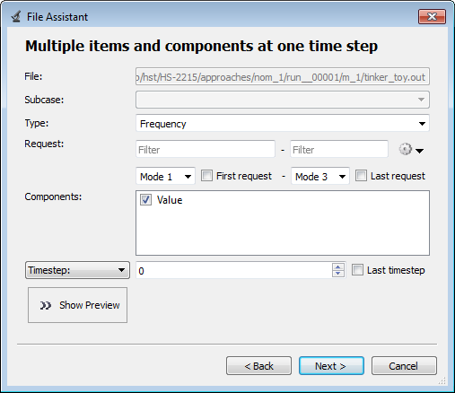
e.	Label the response Frequency_Vector.

f.	Set Expression to None.

hs_2215_8

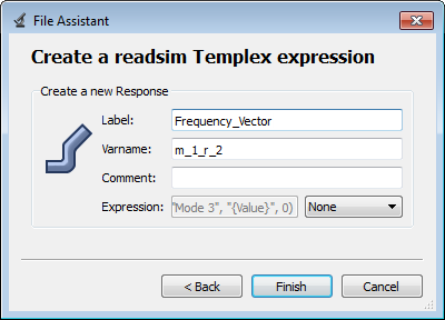
g.	Click Finish. The Frequency_Vector output response is added to the work area.

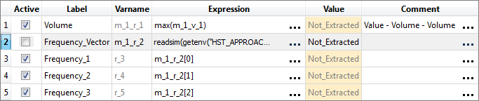
3.	Add three output responses.

a.	Click Add Output Response.

b.	In the Add - HyperStudy dialog, create three output responses labeled: Frequency_1, Frequency_2, and Frequency_3.

4.	Define the Frequency_1 output responses.

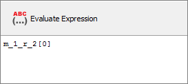
a.	In the Expression column of the output response Frequency_1, click .

b.	In the Expression Builder, click the Responses tab.

c.	Select Frequency_Vector, and click Insert Varname.

d.	In the Evaluate Expression field, append [0] to the end of the expression.

hs_2215_9

Click OK.

5.	Repeat step 4 to define Frequency_2 and Frequency_3, except:

a.	For Frequency_2, append [1] to the end of the expression.

b.	For Frequency_3, append [2] to the end of the expression.

6.	Deactivate the Frequency_Vector output response by clearing it corresponding checkbox in the Active column.

This response will still be calculated and may be referenced by other responses, but it will not saved within HyperStudy.

hs_2215_10

7.	Click Evaluate to extract the output response values.

hs_2215_11

8.	Click OK. This complete the study setup.

1.	In the Explorer, right-click and select Add Approach from the context menu.

2.	In the HyperStudy - Add dialog, select Doe and click OK.

3.	Go to the Specifications step.

4.	In the work area, set the Mode to Modified Extensible Lattice Sequence.

5.	In the Settings tab, change the Number of runs to 4, which is the minimum number of runs for a multivariate effects calculation.

6.	Click Apply.

7.	Go to the Evaluate step.

8.	Click Evaluate Tasks.

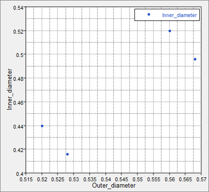
9.	Go to the Post-Processing step, and click the Scatter tab. Using the Channel selector, set the X Axis to Outer_diameter and the Y Axis to Inner_diameter.

All four runs satisfy the constraint, which is inner_radius < outer_radius.

hs_2215_13

10.	Click the Pareto Plot tab, and note which input variables contribute to which output responses.

Above the Channel selector, click and verify Multivariate effects is selected.

hs_2215_14

In this step you will run a second Modified Extensible Lattice Sequence DOE study with 7 new runs, and include the 4 runs from DOE1. This DOE will have a total of 11 runs, which is the default suggested number of runs for a MELS DOE with three input variables.

which is the minimum suggested number of runs for three input variables.

1.	In the Explorer, right-click and select Add Approach from the context menu.

2.	In the HyperStudy - Add dialog, select Doe and click OK.

3.	Go to the Specifications step.

4.	In the work area, set the Mode to Modified Extensible Lattice Sequence.

5.	In the Settings tab:

a.	Change the Number of runs to 7.

b.	Select the Use Inclusion Matrix checkbox.

6.	Import run data from the DOE 1 using an Inclusion Matrix.

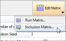
a.	Click Edit Matrix > Inclusion Matrix from the top, right corner of the work area.

hs_2215_12

b.	In the Edit Inclusion Matrix dialog, click Import Values.

c.	In the Import Values dialog, select Approach Evaluation Data and click Next.

d.	Set approach to DOE 1.

e.	Click Next.

f.	Click Finish.

g.	Review the imported run data and click OK.

7.	Click Apply.

8.	Go to the Evaluate step.

9.	Click Evaluate Tasks.

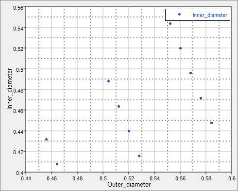
10.	Go to the Post-Processing step, and click the Scatter tab. Using the Channel selector, set the X Axis to Outer_diameter and the Y Axis to Inner_diameter.

Note that all 11 runs still satisfy the constraint, which is inner_radius < outer_radius.

hs_2215_15

11.	Click the Pareto Plot tab, and compare the results to the Pareto Plot from DOE 1.

Note that the magnitude and order of importance has changed in some cases.

hs_2215_16

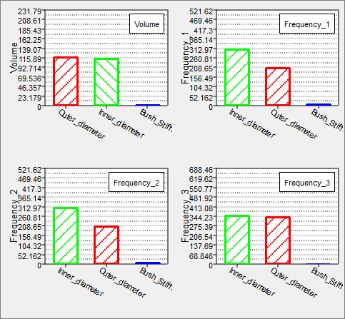
Pareto Plot from DOE2

hs_2215_14

Pareto Plot from DOE1

In this step you will run a third Modified Extensible Lattice Sequence DOE study with 4 new runs, and include the 11 runs from DOE2. This DOE will have a total of 15 runs, which exceeds the number of suggested runs.

1.	In the Explorer, right-click and select Add Approach from the context menu.

2.	In the HyperStudy - Add dialog, select Doe and click OK.

3.	Go to the Specifications step.

4.	In the work area, set the Mode to Modified Extensible Lattice Sequence.

5.	In the Settings tab:

a.	Change the Number of runs to 4.

b.	Select the Use Inclusion Matrix checkbox.

6.	Import run data from the DOE 2 using an Inclusion Matrix.

a.	Click Edit Matrix > Inclusion Matrix from the top, right corner of the work area.

hs_2215_12

b.	In the Edit Inclusion Matrix dialog, click Import Values.

c.	In the Import Values dialog, select Approach Evaluation Data and click Next.

d.	Set the approach to DOE 2.

e.	Click Next.

f.	Click Finish.

g.	Review the imported run data and click OK.

7.	Click Apply.

8.	Go to the Evaluate step.

9.	Click Evaluate Tasks.

10.	Go to the Post-Processing step, and click the Pareto Plot tab. Compare the results to the Pareto Plots from DOE 2.

Note that the results are qualitatively the same, indicating that you will likely have enough runs to draw solid conclusions.

hs_2215_17

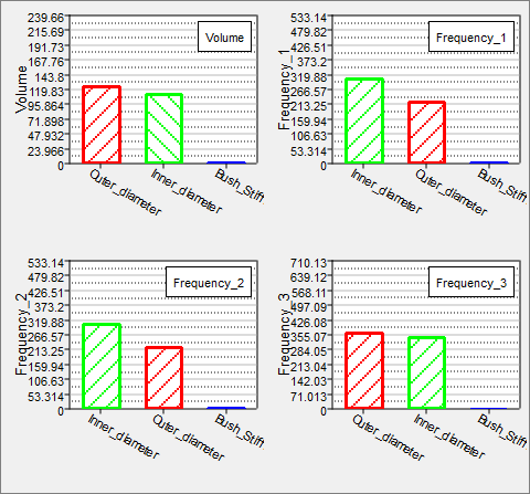
Pareto Plot from DOE3

hs_2215_16

Pareto Plot from DOE2