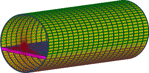
The purpose of this tutorial is to investigate the relative effect of the variable on the identified output responses. Furthermore, this tutorial will demonstrate how to create a Fit in order to investigate combinations of variables that were not explicitly simulated.
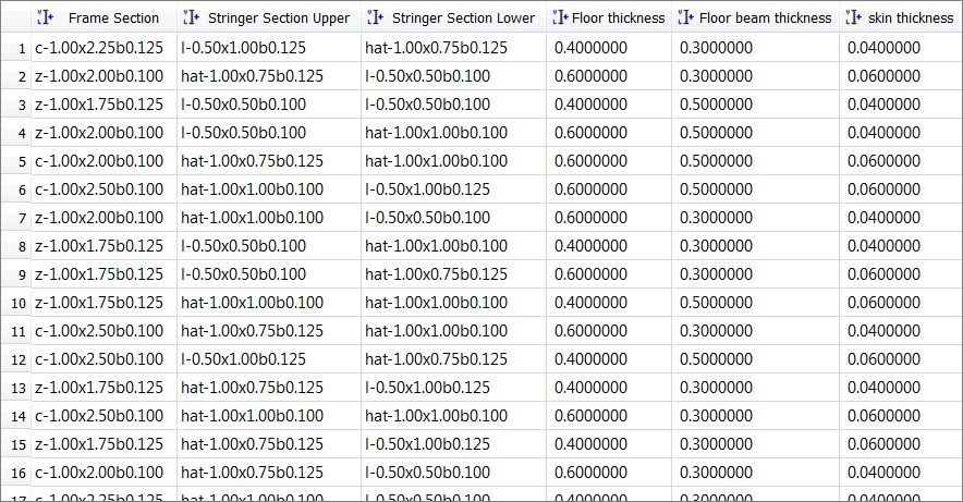
Three continuous variables and three categorical variables are used in this tutorial. The frames can take five possible sections, and the stringers can each take from four available sections.
Continuous variables
| • | Thickness of floor beams |
Category variables
| • | Cross sections of the frames |
| • | Stringers above the floor |
| • | Stringers below the floor |
This tutorial uses three load cases:
| • | Free-free normal modes case |
The files used in this tutorial can be found in <hst.zip>/HS-3010/. Copy the files from this directory to your working directory.
| 2. | To start a new study, click File > New from the menu bar, or click  on the toolbar. on the toolbar. |
| 3. | In the HyperStudy – Add dialog, enter a study name, select a location for the study, and click OK. |
| 4. | Go to the Define models step. |
| 5. | Add a Parameterized File model. |
| a. | From the Directory, drag-and-drop the fuselage.tpl file into the work area. |
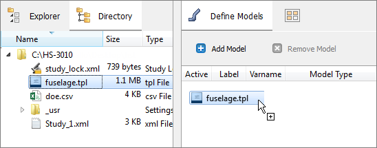
| b. | In the Solver input file column, enter fuselage.fem. This is the name of the solver input file HyperStudy writes during any evaluation. |
| c. | In the Solver execution script column, select OptiStruct (os). |

| 6. | Click Import Variables. Six input variables are imported from the fuselage.tpl resource file. |
| 7. | Go to the Define Input Variables step. |
| 8. | Review the input variable's lower and upper bounds ranges. |
| 9. | Go to the Specifications step. |
|
| 1. | In the work area, set the Mode to Nominal Run. |
| 3. | Go to the Evaluate step. |
| 5. | Go to the Define Output Responses step. |
|
| 1. | Create the Mass output response. |
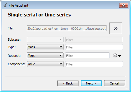
| a. | From the Directory, drag-and-drop the fuselage.out file, located in approaches/nom_1/run_00001/m_1, into the work area. |
| b. | In the File Assistant dialog, set the Reading technology to Altair® HyperWorks® (hgosfreq.exe) and click Next. |
| c. | Select Single item in a time series, then click Next. |
| d. | Define the following options, and then click Next. |
| e. | Label the output response Mass. |
| f. | Set Expression to Maximum. |
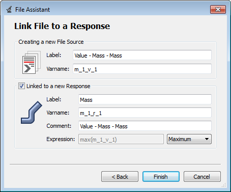
| g. | Click Finish. The Mass output response is added to the work area. |
| 2. | Create two more output responses by repeating step 1, except change the type, request, and component assigned to each output response to the following. |
Because this is a free-free analysis, Freq1 will be the seventh frequency in the list due to the six rigid body modes (all near zero). Freq2 will be the eighth frequency in the list.
Output Response
|
Type
|
Request
|
Component
|
Freq1
|
Frequency
|
Mode 7
|
Value
|
Freq2
|
Frequency
|
Mode 8
|
Value
|
| 3. | Create the Bending displacement output response, which will have a magnitude of node 8196 (loading point). |
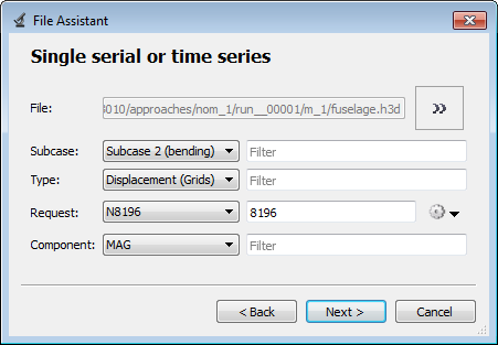
| a. | From the Directory, drag-and-drop the fuselage.h3d file, located in approaches/nom_1/run_00001/m_1, into the work area. |
| b. | In the File Assistant dialog, set the Reading technology to Altair® HyperWorks® (Hyper3D Reader) and click Next. |
| c. | Select Single item in a time series, then click Next. |
| d. | Define the following options, and then click Next. |
| • | Set Subcase to Subcase 2 (bending). |
| • | Set Type to Displacement(Grids). |
| • | For Request, apply a filter of 8196. Press Enter to accept the value entered in the Filter field. |
| e. | Label the output response Bending displacement. |
| f. | Set Expression to Maximum. |
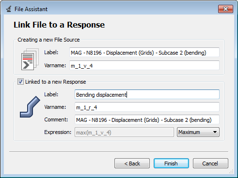
| g. | Click Finish. The Bending displacement output response is added to the work area. |
| 4. | Create the Torsional rotation output response, which will have a z-direction of node 8196 (loading point). |
| a. | From the Directory, drag-and-drop the fuselage.h3d file, located in approaches/nom_1/run_00001/m_1, into the work area. |
| b. | In the File Assistant dialog, set the Reading technology to Altair® HyperWorks® (Hyper3D Reader) and click Next. |
| c. | Select Single item in a time series, then click Next. |
| d. | Define the following options, and then click Next. |
| • | Set Subcase to Subcase 3 (torsion). |
| • | Set Type to Rotation (Grids). |
| • | For Request, apply a filter of 8196. Press Enter to accept the value entered in the Filter field. |
| e. | Label the response Torsional rotation. |
| f. | Set Expression to Maximum. |
| g. | Click Finish. The Torsional rotation output response is added to the work area. |
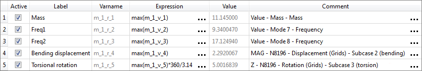
| h. | In the Expression field for Torsional rotation, edit the expression to be max(m_1_v_5)*360/3.14. |
This expression converts the rotation from radians to degrees.
| 5. | Click Evaluate Expressions to extract output response values. |
| 6. | Click OK. This complete the study setup. |
|
| 1. | In the Explorer, right-click and select Add Approach from the context menu. |
| 2. | In the HyperStudy - Add dialog, select Doe and click OK. |
| 3. | Go to the Specifications step. |
| 4. | In the work area, set the Mode to None. |
| 6. | Import run data using the Run Matrix. |
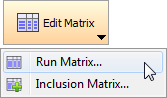
| a. | Click Edit Matrix > Run Matrix from the top, right corner of the work area. |
| b. | In the Edit Data Summary dialog, remove any existing run data. |
| d. | In the Import Values dialog, select Plain Text and click Next. |
| e. | In the Source File field, navigate to the doe.csv file and click Next. |
| g. | Review the imported run data and click Apply. |
| 7. | Go to the Evaluate step. |
| 8. | Click Evaluate Tasks to run the Doe. |
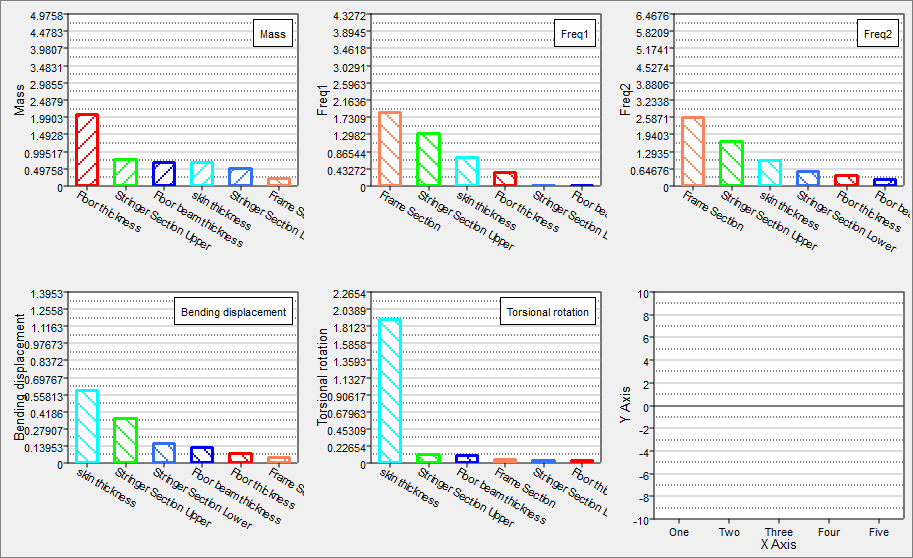
| 9. | Go to the Post Processing step, and click the Pareto Chart tab. Enable multi-plot and select all of the output responses in the Channel selector. If not all of the input variables are plotted, you may need to alter the number of displayed input variables from the options menu. |
The relative effect of a input variable can vary from output response to output response. The most influential input variables when analyzing frequency output responses are Frame Section and Stringer Section Upper. In contrast, the most influential input variables when analyzing the two stiffness conditions are Skin thickness and Stringer Section Upper.
Some input variables can have no effect on output responses. Floor beam thickness has minimal effect on any of the output responses, which indicates that you may want to consider removing this input variable from the analysis.
In a Pareto plot, the effect of input variables on output responses does not measure sensitivity but rather absolute change. Floor thickness has a major effect on Volume. This effect is not a derivative, but a measure of the possible increase over the range of the input variables (the range is the difference between the upper and lower bounds). The floor has a large area and the thickness has very large bounds (+/-0.1 inches), therefore it can make a dramatic impact on Volume as the input variables move through the available space.
|
| 1. | In the Explorer, right-click and select Add Approach from the context menu. |
| 2. | In the HyperStudy - Add dialog, select Fit and click OK. |
| 3. | Go to the Select Matrices step. |
| 5. | In the HyperStudy - Add dialog, add one matrix. |
| b. | Set Matrix Source to Doe1 (doe_1). |

| 8. | Go to the Specifications step. |
| 9. | In the work area, set the Mode to Least Squares Regression. |
| 11. | Go to the Evaluate step. |
| 12. | Click Evaluate Tasks to evaluate the designs. |
| 13. | Go to the Post processing step. |
| 14. | Click the Diagnostics tab to assess the accuracy of the Fit. Select the Mass output response in the Channel selector. |
The R-Square and R-Squared Adjusted values for Mass are 1.00, which indicates the model perfectly predicted the known values.
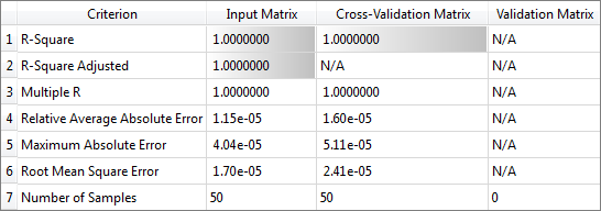
| 15. | Review the diagnostics for the remaining output responses. Notice the R-Squared values are still high, which indicates a high quality fitting of the data. |
| 16. | Click the ANOVA tab and review the Mean Squares Percent column to see the relative importance of input variables. The results should be similar to the results noted in the Pareto Chart tab of the Doe. |
| 17. | Click the Trade-Off tab to perform "what if" scenarios. In the Inputs pane, modify the values of input variables to see their effect on the output response approximations in the Output pane. |
|


