AcuSolve 2017 delivers major improvements in turbulence modeling capability.  This release expands the range of applications that can be simulated with AcuSolve by introducing new physical models, improving on existing models, and providing more user control over the equations that are solved.  The following features are the highlights of the turbulence modeling improvements in AcuSolve 2017.

Addition of Two New Turbulence Transition Models

Turbulent transition plays a major role in the simulation of many engineering applications in which the boundary layer physics dominate the performance of the device.  Examples of these types of applications include flow over airfoils, wings, and turbine blades.  Traditional RANS turbulence models are not capable of accurately predicting the natural transition process that occurs as the laminar boundary layer develops instabilities and becomes turbulent.  In order to properly account for the physics of this process, additional models are necessary.
 
AcuSolve 2017 contains two new turbulent transition models targeted at addressing the issues described above.  Both models rely on a local value of intermittency to determine if the flow is laminar or turbulent, and use this value to control the generation of eddy viscosity.  The most general model is known as the “Gamma-Re_theta” model and represents the earliest published version of a local correlation based transition model.  This model solves for an additional two equations, one representing the intermittency, and the other representing a transition onset criteria that is written in terms of the momentum thickness Reynolds number.  This transition model can be coupled with either the SST or Spalart-Allmaras RANS model.  The second transition model that is available in AcuSolve 2017 is known as the “Gamma” model and represents a simplification of the Gamma-Re_theta closure.  This model eliminates the second equation and solves only for the intermittency transport.  This model may also be paired with either the SST or Spalart-Allmaras turbulence closure.

When selecting the transition/turbulence model combination for a given application it is important to keep in mind the limitations of each one.  Any transition model that is coupled with the Spalart-Allmaras model will be limited in the mechanisms of transition that it can represent.  Because Spalart-Allmaras does not have any mechanism to track local turbulence intensity, it is not possible to accurately simulate bypass transition with this approach.  However, for cases involving natural transition (i.e. relatively low turbulence intensities), the Spalart-Allmaras model provides a robust and computationally efficient modeling approach.  For cases involving bypass transition, it is recommended that the SST model be used with either the Gamma or Gamma-Re_theta transition closure.
 

It should be noted that the calibration of the transition models shipped with AcuSolve are focused primarily for external aerodynamic simulations.  Alternate calibrations will be available in the future that focus on internal flows.  As an interim solution, AcuSolve exposes the correlations used in the transition models via User Defined Function such that users can prescribe their own relationships to control the behavior of the models.

Addition of Three New k-epsilon Turbulence Models

AcuSolve 2017 adds a total of three new k-epsilon based turbulence models to the suite of supported RANS closures.  These models include the realizable k-epsilon model, the RNG k-epsilon model, and the standard k-epsilon model.  All models are fully compatible with AcuSolve’s other features.  The most significant of the changes associated with the k-epsilon turbulence models involves the addition of the dissipation_rate variable and the accompanying wall function.  In contrast to the eddy_frequency variable, the dissipation_rate has very poor numerical behavior near the wall.  To mitigate this challenge, AcuSolve utilizes a two-layer model on the dissipation rate equation.  At low y+ values, the solver uses an algebraic expression to compute the dissipation rate.  As the distance from the wall increases, the solver blends the value of the algebraic expression into the solution of the differential equation, then eventually transitions to using the differential equation solution fully beyond a specific y+.  This two layer treatment produces a robust and stable solution from the k-epsilon models and is the default wall function for all three variants of k-epsilon.  The two layer formulation is valid through the laminar sublayer, and has no lower limit on the y+ value.  However, the upper limit on y+ for the two-layer formulation is on the order of 50.  Users should design their meshes accordingly to avoid models with large y+ values.  This will lead to a degradation in accuracy of the boundary layer profile.

Addition of Menter’s BSL k-omega Turbulence Model

The BSL k-omega model is a two-equation model developed by Menter around the same time that SST was developed.  The BSL model was the original model that proposed a blending of the k-epsilon and k-omega turbulence models to alleviate the sensitivity of the k-omega model to free stream conditions, while still maintaining the accuracy of k-omega in the boundary layer.  The BSL model (or baseline model) shares many common features with SST, with the largest deviation occurring in the expression used to compute the eddy viscosity.  The BSL model does not include the eddy viscosity limiter that SST does.  Although the SST model is expected to provide superior results on separated flows, the BSL model has been added to AcuSolve to provide an alternative to the standard k-omega model.  

Improvements to SST-DES

The SST-DES model in AcuSolve 2017 has been enhanced to include the Delayed Detached Eddy Simulation (DDES) and Improved Delayed Detached Eddy Simulation (IDDES) variants of the model recently published by Menter.  The original zonal formulation of the model is still supported, but no longer the default.  Starting in AcuSolve 2017, the default type of DDES model for SST is the DDES model.  To recover the behavior of previous releases, the zonal version should be used.

Simplified Inputs for Turbulent Simulations

The addition of the new turbulence physics is accompanied by the need to simplify the assignment of inlet boundary values for each of the turbulence model equations.  To accomplish this, the Simple Boundary Condition command has been enhanced to include new methods of assigning inlet boundary values.  The new options expose a set of simplified inputs to users and then automatically compute the inlet boundary values for all active turbulence variables.  The new feature includes a number of automatic options that fully define the turbulence values based on the selection of internal vs. external flow.  Full control over the turbulence values is still available through the direct input method, which was used in previous releases.

Exposure of Turbulence Model Constants

AcuSolve 2017 exposes many new options associated with the suite of turbulence models to users.  To accomplish this, a new command called TURBULENCE_MODEL_PARAMETERS has been introduced.  This command allows control over turbulence model constants, application specific correction terms (i.e. rotation/curvature), wall function types, and variations of a given model to be selected (i.e. IDDES vs. DDES).  This new command introduces a much higher level of control over the turbulence models in AcuSolve than in previous releases, and also migrates some settings that were previously exposed

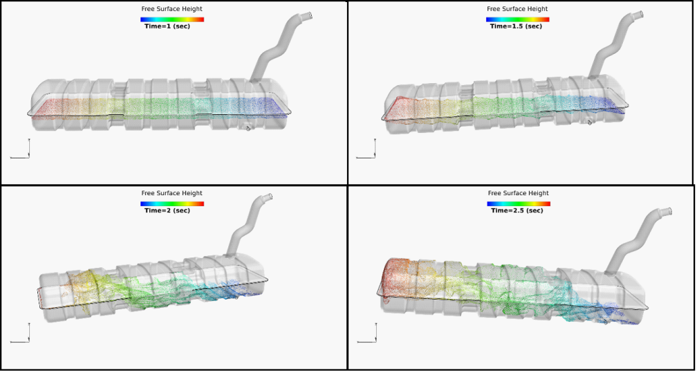
AcuSolve 2017 represents the first release of the solver targeted at the simulation of multiphase flows.  The multiphase flow terminology covers a vast range of applications including bubbly droplet laden flows, slug flows, slurries, fluidized beds, and many more.  AcuSolve’s initial offering within this field is targeted at applications that are typically simulated using a Volume of Fluid (VOF) approach.  These applications include slug flows, free surface flows, and stratified flows.  These applications are characterized by large regions of immiscible fluids in contact with each other.  The interface between the fluids is tracked using an Eulerian interface tracking approach.  This enables the simulation of pouring liquids, free surfaces with large amounts of deformation, bubble entrainment, tank filling/draining applications, tank sloshing applications, and many more.

AcuSolve’s multiphase flow simulation capability enables the simulation of 2 immiscible, incompressible phases.  The initial offering of models supports the simulation of these fluids in combination with heat transfer, turbulence, moving and deforming meshes, non-conformal interfaces, and Fluid-Structure Interaction (rigid body dynamics and flexible bodies).  There is no limit on the density ratio of the two fluids, enabling the simulation of air/water, oil/water, etc.  AcuSolve’s multiphase implementation relies on the same solver as all other features, and retains many of the solver’s beneficial characteristics for transient flow simulations.  Because of AcuSolve’s implicit time integration scheme, multiphase simulations are not restricted to a CFL number of 1.0.  Internal testing of the solver shows stability is retained for interface CFL numbers as high as 20.  Note that the accuracy of the calculation, however, is impacted as the CFL number increases. Best practices for running the multiphase model include the use of isotropic meshes with minimal changes in element size across the interface, and the use of time step sizes that produce CFL numbers on the order of 1 for optimal accuracy.

Examples of multiphase flows that have been solved by AcuSolve include hydraulic oil tank filling, brake bleeding, fuel tank sloshing, and free surface wave applications. This feature is being offered as a beta feature in its first release.  Users are encouraged to experiment with the feature and provide feedback to Altair staff on the performance of the feature.

AcuSolve’s non-conformal mesh interface technology has been improved for the 2017 release.  This release includes changes to the formulation that improve the accuracy of the solution across the interface as well as a number of other enhancements and fixes.

Reformulated Interface Surface Technology

Starting with AcuSolve 2017, users have two options available for the calculation of the flow across non-conformal interfaces.  Both approaches rely on a penalty method for ensuring continuity of the flow across discontinuous interfaces. The newly developed method has proven better at producing smooth solutions across non-conformal mesh interface and retains the robustness and speed of the legacy approach.  When using the new interface formulation, the best results will be achieved when the mesh on all surfaces in contact with each other have the same element size.  This means that the mesh on all touching interfaces should be of constant and uniform size in all directions. The best way to achieve this is to specify a constant surface mesh size on all interface surfaces, then grow a single layer of boundary layer elements off of the interface to ensure consistent height in the surface normal direction.

Support for Deforming and Translating Interfaces

The AcuSolve 2017 release includes an enhancement to the non-conformal mesh technology that enables interface surfaces to be embedded within mesh regions that are undergoing complex rigid body motions as well as local deformation.  This enhancement expands the applications that can be solved using AcuSolve’s moving mesh and interface surface technology such that very complex motions can be simulated by combining these technologies.  An example of where this enhancement is beneficial is when simulating the rigid body motion of a rotor craft with a rotating rotor and pitching blades.  The blades of the rotor can be embedded into a local surface of revolution to handle the changing pitch of the blades, while the entire rotor is embedded in another rotating region that handles the rotation of the rotor about its main axis.

Introduction of “Half-step” Mesh Displacement Output

The 2017 release marks the introduction of the “half-step” mesh displacement output in AcuSolve.  When performing moving mesh simulations, AcuSolve satisfies the equations at the half time steps.  To properly visualize the continuous flow across non-conformal interfaces, it is necessary to visualize the results on the deformed mesh that corresponds to the half time step.  Starting with the 2017 release, this can be accomplished by using the -defcrd command line option to AcuTrans.  When this option is set to endstep, the deformed coordinates that are written to the output file correspond to the coordinates at the end of the step.  When this option is set to midstep, the deformed coordinates correspond to the displacement at the middle of the time step.  The AcuFieldView direct reader has also been modified to allow visualization of the results on the mid step displacement field.  This is accomplished by setting the FV_ACUSOLVE_PREFER_MIDSTEP environment variable to any value.  Note that the mesh displacement vector is still written to disk as mesh_displacement regardless of whether it corresponds to the mid step or end step.

The 2017 release of AcuSolve delivers an expanded documentation offering to provide tools for successfully learning how to use the software, demonstrating the accuracy of the software, and providing an overview of CFD to new users.

Expansion of the AcuSolve Tutorial Manual

The AcuSolve tutorial manual has been expanded to include a total of 19 new tutorial cases.  The newly introduced cases feature tutorials covering the new capabilities of the solver including turbulent transition modeling as well as multiphase flow simulation.  In addition to covering the new features, a collection of tutorials has been added to demonstrate the capabilities of AcuSolve for simulating rotating machinery, free surfaces, heat transfer, and multiphysics applications. As with previous releases, the complete set of input files and documentation for setting up and running the models is included in the AcuSolve installation.

Expansion of the AcuSolve Validation Manual

The AcuSolve validation manual has been expanded to include examples that cover the newly introduced physical models.  In addition to adding cases for turbulent transition and multiphase, additional turbulent simulations have been added to compare the performance of the expanded set of turbulence models.

Addition of the AcuSolve Training Manual

AcuSolve 2017 marks the first release of the AcuSolve Training Manual.  The training manual provides an overview of the theory and background necessary to learn the fundamental concepts associated with performing CFD analysis with AcuSolve.  The training manual includes general theory sessions, as well as exercises that can be used to learn to use AcuSolve.  This manual provides a good overview of CFD and AcuSolve that can be used as a self-paced training

Data Read Controller

The AcuSolve Direct Reader and FV-UNS reader have been updated to give users additional control of how their data is read into AcuFieldView. The readers include the ability to modify the amount of Grid Processing done on the dataset when it is loaded. If users are interested in reading data as fast as possible and reducing memory footprint, selecting Less Grid Processing can reduce the data read time by up to 4x. Selecting More Grid Processing will increase the read time and memory footprint, but leads to increased performance during coordinate sweeps and streamline generation. Selecting Balanced will provide a compromise of both settings. Additionally, the grid processing functionality has been included within the data_input_table for interacting with the data via FVX scripts. The following table summarizes the read performance for the three grid processing options.

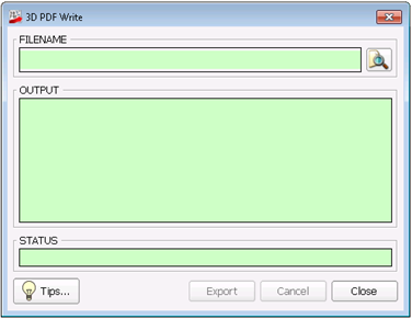
Performance of AcuSolve data read operations using AcuFieldView V14.0 and V2017

3D PDF Export

AcuFieldView is now able to export 3D PDF format files for interactively viewing simulation results directly with Adobe Acrobat Reader versions 10, 11 and DC on Windows systems, and with various reader applications on mobile devices. When users select the 3D PDF Export button, the current window will be exported to a 3D PDF format file. The GUI panel to manage the export process, shown below, is invoked from the Tools menu entry "3D PDF Write..." or alternatively from the 3D PDF icon on the Main Toolbar.

The resulting PDF file contains 3D geometry which may be viewed and rendered with any of the provided controls in 3D PDF viewers. All surfaces, rakes and geometries for all datasets that appear in the current window are exported to the 3D PDF file with several small exceptions. AcuFieldView annotation titles, arrows and legends are exported as data to be rendered on top of 3D objects, for high quality readability. Dataset outlines and axes markers are not exported as the 3D PDF viewer will have its own version of these.

New Vertices Display Types

Two new surface display type options, Vertices and Shaded Vertices, are available for Computational, Iso, Coordinate and Boundary Surfaces. The motivation behind the new types is to provide high performance renderings that bring additional insight for complex Iso-Surfaces and geometries. These new display types provide a great alternate to transparent shaded surfaces for revealing the complexity of internal geometries and convoluted Iso-sur­faces. In addition, they carry information on the local level of mesh refinement.

Data Reader Options Saved as Preferences

Changes made interactively to the "Read Extended Variables” and "Read Duplicate Boundaries" control buttons on the AcuSolve Direct Reader panel are now retained within the AcuFieldView session and saved as preferences.  This change allows AcuFieldView to remember these settings across all sessions run from the same machine.  Saving the size and location of the main window, along with the location of the toolbars (and whether they are docked or not) is part of the broader functionality of saving prefer­ences. This information is stored in FieldView.ini. Its location depends on the operating sys­tem where AcuFieldView is executed from.

Mid Step Mesh Displacement Support in Direct Reader

The AcuSolve Direct Reader now supports mid-step mesh displacement, using the fol­lowing environment variable

FV_ACUSOLVE_PREFER_MIDSTEP

If this environment variable is set to any value prior to launching AcuFieldView, the reader looks for mid-step mesh displacement in the AcuSolve output database. If this is found, it is used to displace the mesh, and imported into the session as the mesh_displacement variable. The follow­ing message is printed to the console:

Displacing mesh coordinates using mid step mesh displacement field.

AcuSolve 2017 contains a number of other notable changes that are worthy of mention.  A brief description of each is shown below:

The following table summarizes the changed or newly introduced AcuSolve input file commands.  Note that a full description of each command is available in the AcuSolve Command Reference Manual.

The following table summarizes the changed or newly introduced AcuSolve command line arguments.  Note that a full description of each option is available in the AcuSolve Programs Reference Manual.