What is the Absolute Nodal Coordinate Formulation?
The Absolute Nodal Coordinate Formulation or the ANCF is a finite element based representation of flexible components in one, two and three dimensions that are allowed to deform under applied load. It is a formulation that allows you to model Non Linear Flexible Element (NLFE) components in your multi-body system. Such flexible components can be used to describe the dynamic motion of deformable bodies. Owing its fully non-linear formulation, this method is capable of handling large deformation as well as large rotation within its elements. The ANCF as implemented in MotionSolve also allows you to model materials with non-linear characteristics like rubber and other hyper-elastic materials.
1.1 BEAM elements
Consider a BEAM12 element as modeled by the ANCF. Such a BEAM element can be considered a LINE element in that it is defined by two nodes – one at the start (g1) and one at the end (g2) of the element. This is illustrated in Figure 1.
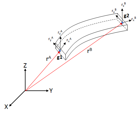
Figure 1: An ANCF BEAM12 element
Unlike traditional finite elements, each grid of a fully parameterized element (like the BEAM12 element), is represented by 12 coordinates. These are:

|
Position of the grid in 3D space.
|

|
Gradient vector in X direction.
|
|
Gradient vector in Y direction.
|

|
Gradient vector in Z direction.
|
Collectively, these are called the nodal coordinates of the beam. The position of the grid is defined in space by the position vector  . The axial strains along the X, Y and Z directions are defined by the magnitude of the gradient vectors. Thus,

|
defines the axial strain in the X direction.
|

|
defines the axial strain in the Y direction.
|

|
defines the axial strain in the Z direction.
|
Further, the shear strain is defined by the angle in between these vectors. As can be seen, a BEAM12 grid then has 12 degrees of freedom:
Degree of Freedom of the grid
|
Rigid translation of the grid along X axis
|
Rigid translation of the grid along Y axis
|
Rigid translation of the grid along Z axis
|
Rigid rotation of the grid about X axis
|
Rigid rotation of the grid about Y axis
|
Rigid rotation of the grid about Z axis
|
Deformation (axial strain) along X axis
|
Deformation (axial strain) along Y axis
|
Deformation (axial strain) along Z axis
|
Deformation (shear strain) in XY plane
|
Deformation (shear strain) in YZ plane
|
Deformation (shear strain) in ZX plane
|
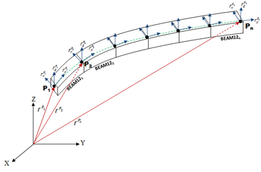
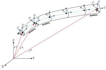
Being fully parameterized, the BEAM12 element is capable of resisting axial, shear, torsion and bending loads. A beam component can thus be modeled using multiple BEAM12 elements as shown in Figure 2.
Figure 2: A beam modeled using multiple BEAM12 elements – using a rectangular and tubular cross-section
The geometric properties of the BEAM12 element can be specified using the PBEAML element which lets you define the cross section of the beam along with the relevant dimensions. In addition to the geometric properties, you also need to specify material properties for the BEAM12 element. The BEAM 12 element supports linear elastic and hyper-elastic models that define the material model. For more information, please refer to the different material property elements in the documentation.
1.2 CABLE elements
The second type of LINE element supported in MotionSolve is the CABLE element. Such a CABLE element can be considered a LINE element in that it is defined by two nodes – one at the start (g1) and one at the end (g2) of the element. This is illustrated in Figure 3.
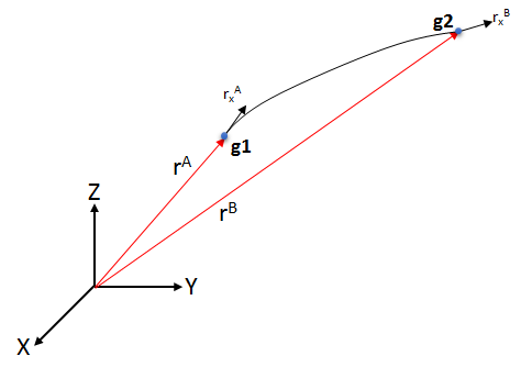
Figure 3: An ANCF CABLE element
Each grid of the CABLE element is represented by 6 coordinates only. These are:
|
Position of the grid in 3D space.
|

|
Gradient vector in X direction.
|
Collectively, these are called the nodal coordinates of the cable. The position of the grid is defined in space by the position vector  . The axial strain along the X direction is defined by the magnitude of the gradient vector. Thus,

|
defines the axial strain in the X direction
|
Based on the construction of this element, it is easy to see that it can only resist axial and bending loads. The cross section of this element is assumed to be constant and does not deform with increasing load.
The CABLE grid then has 9 degrees of freedom:
Degree of Freedom of the Grid
|
Rigid translation of the grid along X axis
|
Rigid translation of the grid along Y axis
|
Rigid translation of the grid along Z axis
|
Rigid rotation of the grid about X axis
|
Rigid rotation of the grid about Y axis
|
Rigid rotation of the grid about Z axis
|
Deformation (axial strain) along X axis
|
Deformation (axial strain) along Y axis
|
Deformation (axial strain) along Z axis
|
A wire or cable component can thus be modeled using multiple CABLE elements as shown in Figure 4.
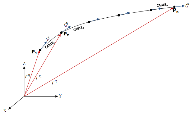
Figure 4: A wire/cable modeled using multiple CABLE elements
The geometric properties of the CABLE element can be specified using the PCABLE element which lets you define the cable cross section area, moment of area and other post processing flags. In addition to the geometric properties, you also need to specify material properties for the CABLE element. The CABLE element supports only the linear elastic material model. For more information, please refer to the documentation.
1.3 Specifying materials for BEAM and CABLE elements
The current implementation of the ANCF supports a variety of material models. The following material types are supported by the ANCF in MotionSolve:
Material Type
|
Element Type
|
Linear elastic (Continuum mechanics and elastic line approach).
|
BEAM12 and CABLE
|
Hyper elastic (Neo-Hookean, Mooney Rivlin and Yeoh).
|
BEAM12 only
|
A linear elastic material typically exhibits the following properties:
| • | The material deforms in a reversible fashion. That is, as soon as the load is removed, it returns to its original shape |
| • | The stress is a linear function of strain |
| • | The strain is not dependent on the loading rate |
The linear elastic material model is defined by three parameters – the Young’s modulus, Poisson’s ratio and the density of the material. This model can be used to model most metals and plastics up until a threshold load beyond which they will start to exhibit plastic deformation and finally yield.
Values for these three material parameters are typically obtained by testing the material in a laboratory. However, owing to the simplicity of this material model, these values are sometimes readily available in textbooks and in engineering handbooks.
A hyper-elastic material model primarily differs from a linear elastic material model in the following ways:
| • | The stress in the material is not a linear function of the strain |
| • | This type of material model is used to model large strains as high as 200% |
Hyper-elastic material models are typically used to model elastomers (like rubber), polymers, foams, biological materials (like muscle) etc. To model such a material, constitutive laws are used which make use of the strain energy density functions. The strain energy density can be thought of the area under the stress-strain curve for any material. For more information on the formulation of the strain energy density function, please refer to the reference manual.
Three such constitutive laws are available with the current implementation of ANCF within MotionSolve:
Type of Material Law
|
Parameters Used to Define the Material
|
Neo-Hookean material law
|
 (Shear modulus) and density (Shear modulus) and density
|
 (Poisson’s ratio) (Poisson’s ratio)
|
 (Density) (Density)
|
Mooney-Rivlin material law
|
 (Material constant) (Material constant)
|
 (Material constant) (Material constant)
|
 (Poisson’s ratio) (Poisson’s ratio)
|
 (Density) (Density)
|
Yeoh material law
|
 (Material constant) (Material constant)
|
 (Material constant) (Material constant)
|
 (Material constant) (Material constant)
|
 (Poisson’s ratio) (Poisson’s ratio)
|
 (Density) (Density)
|
While the Shear modulus, Poisson’s ratio and density parameters may be available in engineering handbooks or textbooks, the material constants for the Mooney-Rivlin and Yeoh material law are determined through lab testing. Typically, uniaxial, biaxial and planar tests are conducted to measure the stresses and strains in the material at different operating points. A curve is then fitted through this data which represents the non-linear relationship between stress and strain. A typical stress-strain relationship for these three material laws is illustrated in Figure 5 obtained through a uni-axial test.
| Note | Hyper-elastic materials are meant for modeling compressive or tensile loads. Applications that involve pure bending may not yield accurate results when using these constitutive models. |
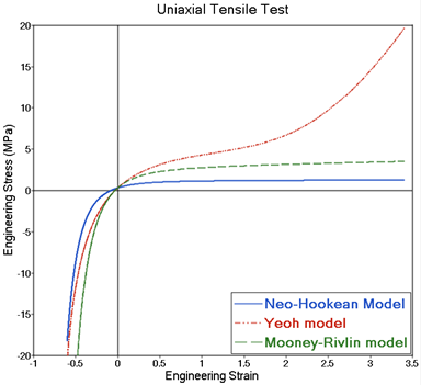
Figure 5: Relationship between engineering stress and engineering strain for hyper-elastic material laws
Which material model should I use?
Depending on the application and the expected strain in the hyper-elastic material, the choice of material laws changes. For applications where a low strain (<10%) is expected, it may be satisfactory to use a linear elastic material. If you are expecting larger strains (for example, while modeling rubber), it is recommended to start with the Neo-Hookean model that is the simplest of the three hyper-elastic models.
If test data is readily available, either the Yeoh or the Mooney-Rivlin model may be used. The choice of which model to use between these two depends on how good of a curve fit is obtained between the material laws and the test data over the range of the strain/stretch that is desired.
MotionView provides a sample set of coefficient values for all three hyper-elastic material models. You may also use your own material constants in MotionView.
2. Pre-processing: Using the ANCF to model flexible components
The implementation of the ANCF in MotionSolve allows you to create flexible components and attach them to the rest of your system in a similar way as rigid bodies.
2.1 Creating flexible components in MotionView
MotionView allows you to create non-linear, flexible components that make use of the ANCF in two ways:
| 1. | By creating atomic components composed of BEAM or CABLE elements. You have to specify the geometric and material properties for the flexible components, and connect these components to the rest of your MBS model. This can be achieved through the Body panel. For more details, please refer to the MotionView documentation on NLFE bodies. |
| 2. | By using the pre-defined sub-systems. In this way, you can create stabilizer bars, coil springs and belt pulley systems with minimal effort. MotionView provides you with a customized GUI for each of these systems that takes care of defining the relevant geometric and material properties as well as creating and assembling the system. |
When using the first method to create NLFE components, you have to specify a list of points for the profile of the BEAM or CABLE that you will create. MotionView fits a cubic spline through these points to generate the NLFE component. As with any cubic spline fitting algorithm, there are certain areas to take care of while specifying the profile points.
Consider, for example, the profile points (in red) as defined in Figure 6 below:
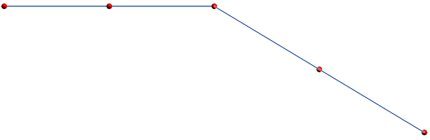
Figure 6: A desired profile for the flexible component
As can be seen, there is a sharp corner in the profile shown above. Using these points as is will result in the following NLFE component:
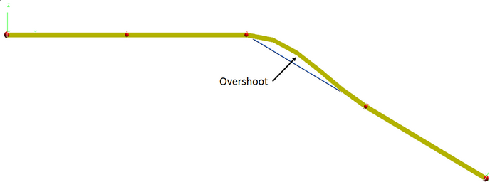
Figure 7: The NLFE component created by using the same profile points shown in Figure 6.
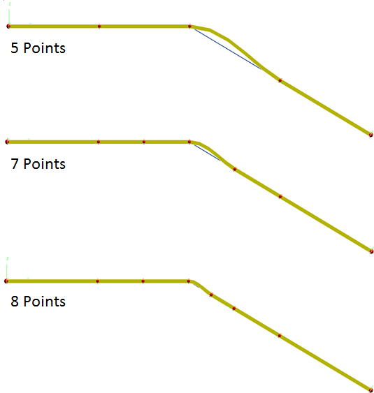
Figure 8: The overshoot is reduced by adding more and more points near the corner
The disadvantage of this approach is that by adding more points, you are creating more BEAM/CABLE elements which will increase the simulation time in general. If you want to avoid doing this, you can make use of the CONN2 connector element that is used to connect structurally discontinuous NLFE elements. In this scenario, you would define two different NLFE components and connect them as shown in Figure 9 below.
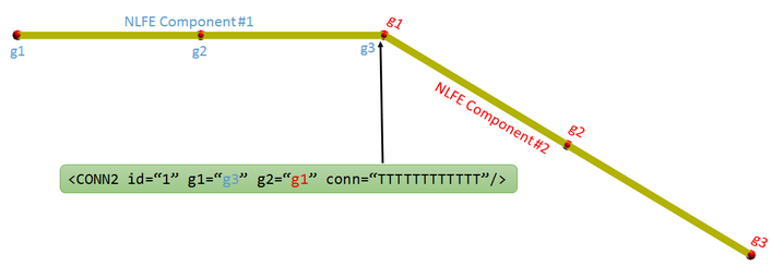
Figure 9: Using a CONN2 element to connect structurally discontinuous NLFE components
2.2 Forces, Joints and Motions with NLFE bodies
MotionSolve supports the use of almost all force, joint and motion types with the NLFE components with the exception of the following:
| 1. | 3D/2D generic contact is currently not supported. |
| 2. | Point to deformable surface contacts and constraints are also not supported |
| 3. | Distributed force application on the NLFE components is not supported |
All the other supported force, joint and motion types are applied to the NLFE component via the use of markers. For example, consider the case where an NLFE cantilever beam is fixed to the ground at one end (Figure 10). A fixed joint is created between one end of the beam (NLFEBody 0) and the ground (Ground Body). In doing so, a marker is automatically created and attached rigidly to the NLFE body at the point of attachment (beam_ground).
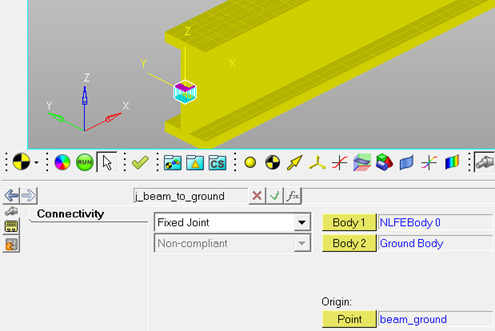
Figure 10: A cantilever beam fixed to ground via a FIXED joint
This marker will be rigidly attached at the corresponding grid of the NLFE component. “Rigidly” here means that 6 degrees of freedom of the grid are arrested – these are the X, Y and Z translation of the grid, as well as the relative rotation of the grid with respect to the marker about the X, Y and Z axes. However, as is noted in Section 1.1, this leaves 6 degrees of freedom (lengths of the gradient vectors in the X, Y and Z direction, as well as the angle between the three gradient vectors) for the BEAM grid. These are not constrained and are allowed to change. This results in the following scenario:
Degree of Freedom of the grid
|
Constrained?
|
Rigid translation of the grid along X axis
|
Yes
|
Rigid translation of the grid along Y axis
|
Yes
|
Rigid translation of the grid along Z axis
|
Yes
|
Rigid rotation of the grid about X axis
|
Yes
|
Rigid rotation of the grid about Y axis
|
Yes
|
Rigid rotation of the grid about Z axis
|
Yes
|
Deformation (axial strain) along X axis
|
No
|
Deformation (axial strain) along Y axis
|
No
|
Deformation (axial strain) along Z axis
|
No
|
Deformation (shear strain) in XY plane
|
No
|
Deformation (shear strain) in YZ plane
|
No
|
Deformation (shear strain) in ZX plane
|
No
|
Rigid translation of the grid along X axis
|
No
|
The effect of the un-constrained additional 6 DOFs may become noticeable in some scenarios. For example, consider the same cantilever beam subjected to an end load of 100 kg-force. The deformation of the fixed end of the beam is visualized in Figure 11. The grey feature lines represent the model configuration or the configuration at time = 0.
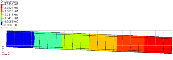
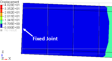
Figure 11: Deformation of the cantilever beam under an end load
Looking closely at the end where the beam is fixed to the ground (Figure11), it seems that the beam cross-section has rotated about the Y axis. This seems to be the wrong behavior, since the beam was fixed to ground and so should not rotate about any axis.
The reason the beam appears to rotate about the Y axis in this case is because of the additional 6 DOFs that are not constrained by the fixed joint. Due to this, the gradient vectors of the beam at the fixed end are free to stretch and twist relative to each other. This can be confirmed by plotting the gradient vectors at the start of the beam in the direction along the beam and normal to it.
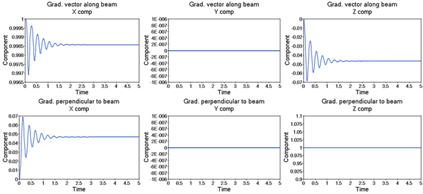
Figure 12: The gradient vector along and normal to the beam at the fixed end
As can be seen from the plot above, the gradient vector along the beam changes from (1,0,0) to ~(0.998574, 0, -0.0466717). Since the NLFE elements are drawn such that the gradient vector along the beam axis is always normal to the element, this results in what looks like a rotation of the beam cross section at the start.
To alleviate this, you need to “fully” clamp the grid at the fixed end of the beam to the ground. This is achieved by using the CONN0 element. The CONN0 element is a connector element that allows you to rigidify the gradient vectors of a single grid. Please see the NLFE reference manual for more information on this.
For this model, adding the CONN0 element, and “fully” clamping the grid at the fixed end of the beam to the ground results in the expected simulation result shown in Figure 13 below.
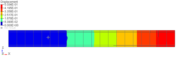
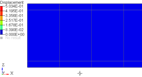
Figure 13: Deformation of the cantilever beam under an end load with the CONN0 element
Further, the gradient vectors at the fixed end also do not change during the simulation, as is expected while fixing the beam to the ground at this end.
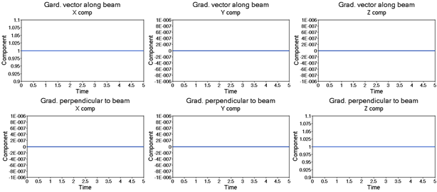
Figure 14: The gradient vector along and normal to the beam at the fixed end with the CONN0 element
| Note | MotionView provides a system definition for easy creation of the CONN0 element that can be imported into your model. This way, you do not have to hand-edit the XML deck. |
2.3 Specifying pre-load in your flexible components
The ANCF formulation in MotionSolve lets you specify two sets of positions for each grid that makes up the flexible component:
| 1. | The model or loaded configuration. This set of nodal coordinates defines the loaded or model configuration. In this configuration, you can specify the following: |

|
The position vector at the loaded/stressed configuration.
|
|
The gradient vector in X direction at the loaded/stressed configuration.
|

|
The gradient vector in Y direction at the loaded/stressed configuration.
|
|
The gradient vector in Z direction at the loaded/stressed configuration.
|
| 2. | The unloaded or relaxed configuration. This set of nodal coordinates defines the unloaded or relaxed configuration. These are denoted in the ANCF XML file by a suffix “0” after each attribute, for example, x0, y0, z0 and so on. In this configuration, you can specify the following: |
|
The position vector at the unloaded/relaxed configuration.
|
|
The gradient vector in X direction at the unloaded/relaxed configuration.
|
|
The gradient vector in Y direction at the unloaded/relaxed configuration.
|
|
The gradient vector in Z direction at the unloaded/relaxed configuration.
|
| Note | If the unloaded/relaxed configuration is not specified, MotionSolve assumes that the loaded configuration is identical to the unloaded configuration, thereby the structure is not pre-stressed. This is also the case if the unloaded configuration is identical to the loaded configuration. |
As an example, consider a beam of circular cross section fixed at both its ends and subjected to a center load. The unloaded configuration is specified as the configuration when the load is not present or equal to zero.
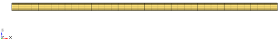
Figure 15: The unloaded or no load configuration
The loaded configuration (Figure 16) is specified as the configuration when the beam is under maximum deformation. A center load of 1000N is applied in this case.
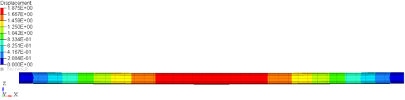
Figure 16: The loaded configuration. Shown here are the displacement contours.
Thus, the loaded and unloaded configurations in the ANCF XML file are specified as follows (this is illustrated for the middle grid, in the interest of saving space):
<GRID
id="301008"
x0="500.000000" y0="0.000000" z0="0.000000"
rx0="1.000000 0.000000 0.000000"
ry0="0.000000 0.000000 1.000000"
rz0="0.000000 -1.000000 0.000000"
x="5.0000000E+02" y="2.2342947E-09" z="-1.8751877E+00"
rx="1.0000086E+00 1.8714474E-15 1.4090006E-17"
ry="-1.3419917E-17 -1.2981139E-09 9.9999766E-01"
rz="1.8569096E-15 -9.9999740E-01 -1.3584520E-09"
/>
|
As can be seen, the loaded and unloaded nodal coordinates are different. The difference between the loaded and unloaded “z” positions represents the maximum deformation of this beam in this case.
This method can thus be used to represent pre-stressed components in your model. For such scenarios, MotionSolve calculates the stress in the component based on the difference between the loaded and unloaded configuration, which can be used to model pre-stress in the flexible component. For the component defined above, the “pre-stress” in the beam at t=0 is illustrated in Figure 17 below.
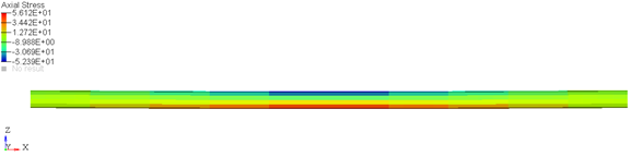
Figure 17: The stress at t=0 calculated due to the difference in loaded and unloaded configurations. Shown here are the axial stress contours.
3. Solving: Solving models with NLFE components
MotionSolve supports the following analysis types when modeling flexible components using the ANCF:
Linear analysis is currently not supported with the NLFE components.
3.1 Static and Quasi-Static analysis
Both CABLE and BEAM NLFE components are supported for Static and Quasi-Static analyses. You may choose any of the available material models while defining the BEAM or CABLE components for these analyses. There are a few key points that must be kept in mind while trying to simulate models containing NLFE components through a static or quasi-static analysis:
Applying motion
Any applied motion must be applied slowly, preferably through the use of a STEP function to ensure that the analysis is successful. This is because in a static/quasi-static analysis, there are no inertial effects and so the displacement of an NLFE grid between two consecutive static steps is not limited by inertia or material properties. What this means is that if the motion is applied suddenly and in one shot, the analysis can result in wrong results or fail altogether. This is a good modeling practice not just for NLFE bodies, but for most MotionSolve models subjected to a static/quasi-static analysis
Further, a static simulation of your model is not successful, you may try to switch to a quasi-static analysis and apply any actuation motions using a STEP function, if applicable.
Reference Length
A good modeling practice is to setup your model for a static analysis such that the maximum displacement of any NLFE grid is not more than a reference length in each static iteration. A good reference length for your NLFE components(s) is the minimum length or span of a beam element, for example. The choice of this reference length depends on the model being simulated.
The above criteria can be enforced by
| • | Constraining your NLFE component(s) suitably such that large displacements are avoided |
| • | Switching to a quasi-static analysis if large displacements are expected. This enables you to specify the step size which in turn will allow you to wield control over the displacements during the static analysis |
3.2 Transient analysis
Both CABLE and BEAM NLFE components are supported for transient analyses as well. At this time, only the DAE integrator DSTIFF is supported for transient solutions. As with static analysis, you may choose any of the available material models while defining the BEAM or CABLE components for these analyses.
As with the static analysis, there are a few recommendations while running simulations with NLFE components that will ensure a successful simulation.
Specifying damping
The NLFE components at this time do not support physical damping for the structure. However, MotionSolve does provide a numerical damping parameter that can be used to mimic physical damping in some cases. This damping is specified by multiplying a damping factor (provided by the user) with the stiffness matrix. As with any damping factor, it is recommended to start with a factor of 0 and ramp it up till the desired behavior is achieved.
True physical damping will be implemented for the NLFE structural components in future releases.
Shown in Figure 18 below is a comparison of the end deflection of a cantilever beam under end loading for different damping factor values.
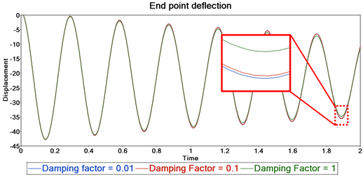
Figure 18: The displacement for different damping factors
Maximum order used for the simulation
Models containing NLFE components typically are very numerically stiff. This may cause numerical convergence issues if trying to solve the model with a large integration order like 5, for example. It is recommended to use a maximum order of 1 or 2 for solving models that contain NLFE components. The maximum order is specified by the attribute max_order in the Model/Command statement <Param_Transient>.
4. Post-processing: Generating results for NLFE components
You can post-process the NLFE components in your model in the same way you would a CMS flexible body.
| Note | There is an important difference while post processing NLFE components as compared to CMS flexible bodies. Unlike CMS flexible bodies, the NLFE body is always represented in global coordinates. As a result of this, there is no floating marker or local part reference frame (LPRF) that moves with the flexible component. A direct consequence of this is that one cannot view the contours of deformation for the NLFE component. This is a result of the design of the ANCF technology. |
There are three types of results available for the NLFE component:
Results in the MRF/ABF output files
The output MRF/ABF file contains the following signals for each grid of each NLFE component in your model:
Y component
|
Description
|
DX, DY, DZ
|
Grid X, Y and Z positions.
|
UVX(1), UVX(2), UVX(3)
UVY(1), UVY(2), UVY(3)
UVZ(1), UVZ(2), UVZ(3)
|
X, Y and Z components of the gradient vectors in the X, Y and Z directions
|
VX, VY, VZ
|
Grid velocity in the X, Y and Z directions
|
WX, WY, WZ
|
Grid rotational velocity about the X, Y and Z axes
|
Note, all of these are with respect to the global or ground frame, owing to the formulation of the ANCF.
Marker based results in the MRF/ABF/PLT
In addition to the above results, you may also use any marker based request on the NLFE component by attaching the marker to a grid on the NLFE component. For example, you may use expressions like DM(), VM() and any other marker based expression requests. These requests will be written out to all the output files including the MRF, ABF and the PLT.
Visualizing stress, strain and displacement
For each NLFE component (composed of BEAM and/or CABLE elements) in your model, MotionSolve writes out a 3D representation in the H3D file. Using the H3D file in HyperView, you are able to visualize component stresses, strains and displacements in addition to animating the simulation. Figure 19 below illustrates this.
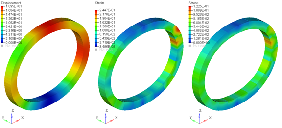
Figure 19: Displacement, Strain and Stress contours
Note that the stresses/strains are calculated at the centroid of each element segment for both the BEAM and CABLE elements. The displacements, however, are calculated at all the nodes that are used to construct the three dimensional representation of the BEAM/CABLE. Owing to this difference and depending on the number of elements and segments in your NLFE component, the stress/strain contours may appear to be discontinuous while the displacement contours appear continuous when plotted in HyperView.
To capture more accurate stress/strain contours, you may use one or more of the following methods:
| 1. | Increase the number of NLFE sub-segments in your component. This leads to a finer discretization of the element shape and therefore the stresses are more accurate. Increasing the number of segments for your NLFE component will increase the post-processing time for your results. The solution time, however, should remain unaffected. |
| 2. | Make use of stress averaging tools within HyperView. These are accessed in the Contour panel within HyperView. Using this method does not increase the post-processing or solution time in MotionSolve, since the averaging is done within HyperView with the available results in the animation H3D. |
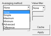
Figure 20: Contour averaging options in HyperView
Below is an example of plotting stress contours with and without stress averaging:
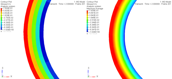
Figure 21: A stress contour of the same NLFE component with stress averaging OFF (left) and ON (right)
| 3. | Increase the number of elements in your NLFE component by defining more grid points. Although this is the most effective way to increase the accuracy of the stresses/strains, doing this also has the most severe effect on both the solution time and the time spent post-processing in MotionSolve. This option should only be used if the above two options do not give you satisfactory results. If you do increase the number of elements in your component to get more accurate stresses, you may consider doing so only in the areas of interest – for example, in curved sections of your component, or where stress concentrations are likely to occur. |
5. Frequently asked questions (FAQs)
Q. Can I model non-linear bending of beam like components?
A. Yes, you can model the non-linear bending of a beam up until the material’s elastic load limit.
Q. My model fails to solve, what are some areas I can look at?
A. If your simulation fails, please try one of the following:
| • | Reduce the maximum order of the integrator to 1 or 2 |
| • | Remove any damping factors specified for the NLFE components (set them to zero). |
| • | Try to increase the number of elements in your NLFE component |
| • | If you are modeling hyper elastic materials, you may want to try using the Neo-Hookean model before using the Yeoh or Mooney-Rivlin as these are more sensitive models and require accurate material constants from test data. |
Q. I attached my NLFE body to a fixed joint, but it does not behave as if it is fixed. What is going on?
A. Please see Section 2.2 above.
Q. How can I contour the deformations for my NLFE component?
A. Currently, you cannot. Please see Section 4 above.