Modeling Constraints

Constraints arise when the motion of a body is restricted by connections to other bodies. For example, when two bodies are connected by a ball and socket joint, they can only rotate with respect to each other. The relative translational degrees of freedom are eliminated by the ball and socket joint. The bodies are said to be constrained by the ball and socket joint. Mathematically, the ball and socket joint manifests as an algebraic equation called the constraint equation.

Constraints are classified in several ways. One key classification is based on whether the constraint depends explicitly on time. Constraints without explicit time dependence are used to model joints, such as the ball and socket joint and the universal joint. Constraints with explicit time dependence are used to represent prescribed motions into the system, such as the constant speed spinning motion of a turbine. For other classifications, refer to dynamics textbooks, such as Advanced Engineering Dynamics by J. H. Ginsberg.

Each constraint introduces, internally, constraint forces and/or moments that enforce the algebraic relationship implied by the constraint. These constraint forces and moments can be computed using MotionSolve to obtain the loads acting through the connections in your mechanism. In the case of prescribed motions, the constraint forces provide driving forces and moments which are useful in estimating the capacity required of actuators to achieve those motions.

Joints are models of interconnections between machine components. Perhaps the most familiar example is a door hinge which may be modeled as a revolute joint. This joint has only one degree of freedom corresponding to the rotation about the joint axis.

The following table shows the various constraints types and the number of constraint equations they contribute.

Constraint Type	Translational Constraints	Rotational Constraints	Total Constraints
Constraint_Coupler			1
Constraint_CVCV			3
Constraint_CVSF			1
Constraint_Gear			1
Constraint_Joint:CONSTANT_VELOCITY	3	1	4
Constraint_Joint: CYLINDRICAL	2	2	4
Constraint_Joint: FIXED	3	3	6
Constraint_Joint: FREE	0	0	0
Constraint_Joint: INLINE	2	0	2
Constraint_Joint: INPLANE	1	0	1
Constraint_Joint: ORIENTATION	0	3	3
Constraint_Joint: PARALLEL_AXES	0	2	2
Constraint_Joint: PERPENDICULAR	0	1	1
Constraint_Joint: PLANAR	1	2	3
Constraint_Joint: RACK_PINION			1
Constraint_Joint: REVOLUTE	3	2	5
Constraint_Joint: SCREW			1
Constraint_Joint: SPHERICAL	0	3	3
Constraint_Joint: TRANSLATIONAL	2	3	5
Constraint_Joint: UNIVERSAL	3	1	4
Constraint_PTCV			2
Constraint_PTSF			1
Constraint_SFSF			1
Constraint_PTDCV			2
Constraint_PTDSF			1

These joints are also called "configuration constraints" because they can be expressed purely in terms of the configuration of the system without requiring the velocity terms. Further, they are not a function of time. Such constraints are also called "workless constraints" because they do not add or remove energy from a system.

Note that joints provide great computational efficiency in simulating complex mechanical systems, such as a full car or truck assembly precisely by "idealizing away" effects, such as clearance and friction. However, these effects may be important in some cases. MotionSolve allows you to model these effects in other ways. For example, to model clearance, you may replace the joint with a contact force element. To model friction in a joint, you may use a force or torque as a function of joint reactions and kinematics.

Much like joints, motions are an idealized representation of actuators. They constrain some degrees of freedom to vary as a specified function of time. The corresponding constraint force is the effort required to produce the motion. Motions may add or remove energy from a system.

It is possible for you to "over constrain" a system by adding too many constraints. The door is a typical example of an over constrained system. A typical door has three hinges connecting it to the door frame. When the hinge is represented with a revolute joint, only one hinge is needed in the model. The hinge is idealized and it cannot deform or bend. The other two hinges are "redundant" because they do not add any new information to the system. Mathematically, the two sets of constraint equations contributed by the other two hinges are indistinguishable from the set contributed by the first one.

This redundancy manifests itself as a rank-deficiency in the matrices that are internally generated by MotionSolve, which means that there is no unique solution to the problem as posed. Instead of exiting at this point with an error, MotionSolve is designed to detect this condition and automatically remove the redundant constraints so that a unique solution can be found and the simulation can proceed.

In such a scenario, MotionSolve writes out a warning message like the one shown below:

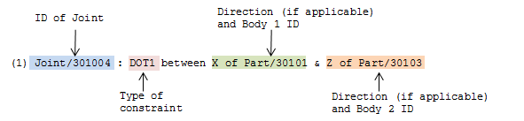
WARNING: The following redundant constraints were removed:

-------------------------------------------------

(1) Joint/301004 : DOT1 between X of Part/30101 & Z of Part/30103

(2) Joint/301004 : SPH_Y between Part/30101 & Part/30103

(3) Joint/301002 : DOT1 between Y of Part/30102 & Z of Part/30104

-------------------------------------------------

NOTE: DOT1 is the perpendicular constraint between two axes.

DOT2 is the perpendicular constraint between an axis and a vector rj->ri.

SPH_X(or Y,Z) is the coincidental constraint between the X(or Y,Z) of two points.

DIST is the distance constraint between two points.

The existence of redundant constraints may indicate potential modeling errors.

See Users Manual for further info and remarks.

The warning statement above is explained in the picture below:

modeling_constraints_fig1

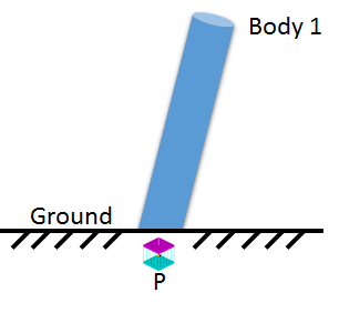
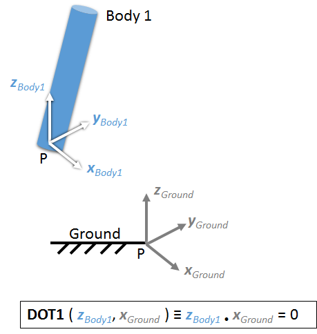
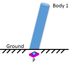
Depending on the joint which has the redundant constraint, the type of constraint is one of the following:

DOT1

This constraint is defined between two vectors. Each vector is an axis that belongs to a marker that is attached to each body. This constraint requires the two axes to be perpendicular to each other. This constraint is used in a number of joints in MotionSolve including the fixed joint, revolute joint, and cylindrical joint, for example. As an example, the DOT1 constraint is illustrated in Figures 1 and 2 for a fixed joint between two bodies.

modeling_constraints_fig2

Figure 1: Body 1 is attached to ground using a fixed joint at point P

modeling_constraints_fig3

Figure 2: DOT1 constraint between z axis on Body 1 and x axis on Ground

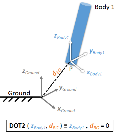
DOT2

This constraint, like DOT1, is defined between two vectors. One vector is an axis that belongs to a marker that is attached to one body. The other vector is defined in between the two bodies. This constraint requires the two vectors to be perpendicular to each other. This constraint is used in a number of joints in MotionSolve including the planar joint, inline joint, and inplane joint, for example. As an example, the DOT2 constraint is illustrated in Figures 3 and 4 for an inplane joint between two bodies.

modeling_constraints_fig4

Figure 3: Body 1 is attached to ground using an inplane joint at point P

modeling_constraints_fig5

Figure 4: DOT2 constraint between z axis on Body 1 and vector from Body1 marker origin to Ground marker origin

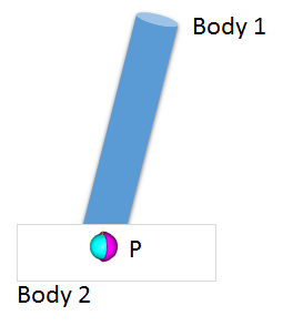
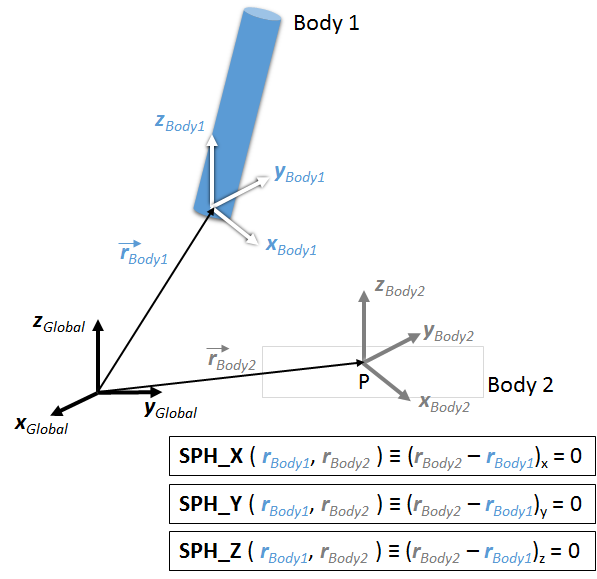
SPH_X, SPH_Y, SPH_Z

The spherical constraint also acts between two markers. This SPH_X, SPH_Y, and SPH_Z constraints require that the X, Y, and Z positions of the two marker origins be the same respectively. One or more of these constraints are used in the fixed joint, ball joint, and revolute joint, for example. This is illustrated in Figures 5 and 6 for a spherical or ball joint.

modeling_constraints_fig6

Figure 5: Body 1 is attached to Body 2 using a ball joint at point P

modeling_constraints_fig7

Figure 6: SPH_X, SPH_Y and SPH_Z constraints between the position vector of two markers

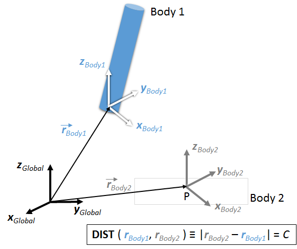
DIST

This constraint, like the SPH_* constraint also prescribes the distance between the origins of two markers. The DIST constraint requires that the magnitude of the difference between the position vectors of the two markers’ origins be equal to a certain value. In the case that this value is equal to zero, this constraint becomes equivalent to the SPH_X, SPH_Y, and SPH_Z constraints combined. This is illustrated in Figure 7.

modeling_constraints_fig8

Figure 7: DIST constraint between the position vector of two markers

To further illustrate the use of these constraints, the table below describes how these constraints are used to model common joints between bodies.

Constraint Type	Description	Type of joint
SPH_X, SPH_Y, SPH_Z	Constrain 3 Translational Displacements	Fixed Joint
3 DOT1	Constrain 3 Rotational Displacements	Fixed Joint
SPH_X, SPH_Y and SPH_Z	Constrain 3 Translational Displacements	Ball or Spherical Joint
SPH_X, SPH_Y and SPH_Z	Constrain 3 Translational Displacements	Revolute Joint
2 DOT1	Constraint 2 Rotational Displacements	Revolute Joint

However, note carefully that the constraint forces corresponding to the removed constraints are reported as zero (no constraint, no force). This implies that other joints in your mechanism may have unrealistically high constraint forces and/or moments. If you intend to use your model to obtain realistic constraint forces, then you must follow one of these approaches:

1.	Select the constraint types in such a way as to ensure that no redundant constraints are present.

2.	Replace idealized joints with force/torque-based connections (for example, bushings).

3.	Model the flexibility of the parts on which the joints act. By replacing rigid bodies with flexible bodies, more degrees of freedom are introduced, which may eliminate the redundancy of the joint equations that act on this part.