Modeling in MotionSolve

The modeling process begins with the idealization of a system as an assembly of more basic components. For example, under certain circumstances, it is possible to replace an entire powertrain with a few differential equations. The choice of simplifying assumptions can have a significant effect on the usefulness and validity of the results, and on the cost of creating and maintaining the models. A realistic idealization of the physical model, therefore, is very important.

The desired results define the purpose of the model. You should decide on the physical behavior of interest, the simulations that should be performed, the required outputs, and the required degree of accuracy. Once the purpose of the model is defined and the necessary degree of complexity is determined, the model is decomposed into an appropriate set of basic components. Decomposition permits a crawl-walk-run approach to model building. Simple models are first built and tested. Complexity is gradually added as model confidence grows.

MotionSolve normally requires the following data to specify the mechanical model for a simulation:

•	The mass and inertia of the components.

•	The geometrical properties of the system including the location of the center of mass for each component, the location of joints that connect the system, and the points at which the specified motion functions and forces apply.

•	The geometrical shape of the bodies when contact between parts is important.

•	The connectivity for the system (the mechanisms for connecting the parts) defined in terms of mechanical joints, higher-pair contacts, other constraints, and elastic elements.

•	A description of the external forces and excitations acting on the system.

Inertia bearing elements (parts) are typically represented in the following ways:

•	Rigid bodies: Generally characterized by three translational and three rotational degrees of freedom.

•	Flexible bodies: Generally represented in the modal domain using component mode synthesis.

•	Point masses: Characterized by three translational degrees of freedom.

•	2D rigid bodies: Generally characterized by two translational and one rotational degree of freedom.

•	2D/3D mixed bodies: Used for example, to model belts where torsional motion of the belt is not generally of interest.

Once the parts representing a system are created, they need to be constrained with each other or to a global coordinate system (often referred to as ground). A large library of constraints is available for this purpose. Some typical constraints are:

•

Lower pair standard joints: Figure 1 shows some commonly used joints. Physically, a lower pair joint consists of two mating surfaces that allow relative translational and/or rotational movement in certain specific directions only. The surfaces are abstracted away, and the relationships are expressed as a set of algebraic equations between points and directions on two bodies.

lower_pair_joint_ex

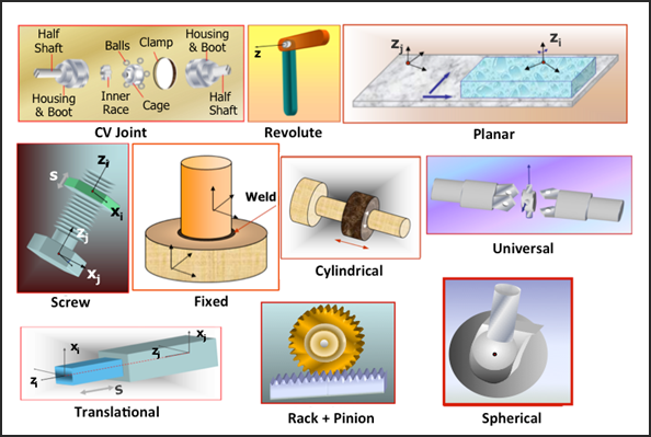
Figure 1 - Examples of lower pair joints

•	Joint primitives: These are abstract entities that enforce specific constraint relationships. See Figure 2 for some of the commonly used joint primitives.

joint_primitives_ex

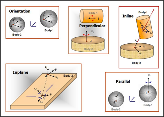
Figure 2 - Examples of joint primitives

•	Higher pair joints: These are constraints involving curves and surfaces. Examples of higher pair constraints include point-to-curve, curve-to-curve, curve-on-surface and surface-on-surface. Curves and surfaces are typically defined parametrically. See Figure 3 below for examples.

parametric_curves_ex

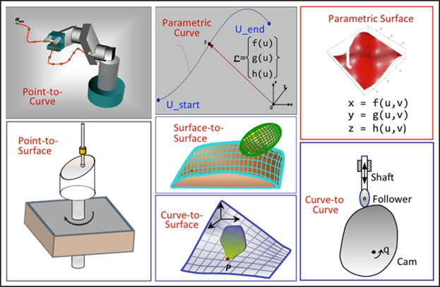
Figure 3 - Examples of parametric curves, surfaces and higher pair joints

•

Motions, Coupler and Gear constraints: A motion constraint defines an input excitation between two coordinate systems in a model. The motion input may be translational or rotational. An expression defines the motion characteristic. A coupler constraint defines an algebraic relationship between the degrees of freedom of two or three joints. This constraint is used to model idealized spur gears, rack and pinion gears, differentials, and hydraulic cylinders. See Figure 4 for some common examples of these.

motion_coupler_gear_ex

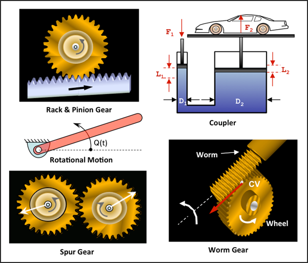
Figure 4 - Examples of Motion, Coupler, and Gear elements

•

Forces and Flexible connections: Parts can be connected not only through constraints but also with force elements. Constraints define algebraic relationships in the system; these represent workless, idealized connections. In contrast, flexible connections are modeled with force elements. Force elements may act between two or more parts; they can be translational or rotational; they can have an action-only or action-reaction characteristic. Very often, they depend nonlinearly on the system displacements, velocities, and other states in the system. Sometimes forces, especially those experimentally measured, are expressed as functions of time. Examples are the aerodynamic force acting on airplane wings and the road loads imposed by the road on the spindles of a vehicle. All MBS tools support a large set of force connectors. Figure 5 shows examples of force connectors.

force_elements_ex

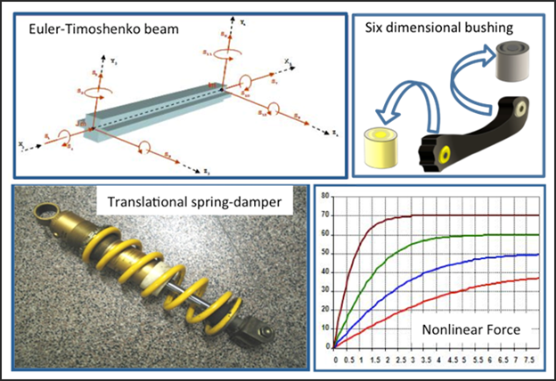
Figure 5 - Examples of force elements (Spring-Damper, obtained from http://it.wikipedia.org/wiki/File:Ammortizzatore.jpg, (last visited November 29, 2009))

•	Timoshenko beams: Beams modeled according to the equations developed by the Ukrainian/Russian-born scientist.

•

Bushings: This element defines a linear force and torque acting between two coordinate systems belonging to two different parts. The force and torque consist of: a spring force, a damping force, and a pre-load vector. Bushing elements are typically used to reduce vibration, absorb shock, reduce noise, and accommodate misalignments.

•	Fields: This is a generalization of a bushing. It can be linear or nonlinear.

•	Spring dampers: The element defines a spring and damper pair acting between two coordinate systems. The element can apply a force or a moment. The force is characterized by a stiffness coefficient, a damping coefficient, a free-length, and a preload.

•

General forces: These can define a single component of a force or torque, or the force and/or torque vector acting between two bodies. The components may be defined as function expressions in the input file or via user-written subroutines. The components can be a function of any system displacement, velocity, or any other state variable in the system.

•

Rigid-rigid contact: This defines a 3-D contact force between geometries on two rigid bodies. Whenever a geometrical shape on the first body penetrates a geometrical shape on the second body, a normal force and a friction force are generated. The normal force tends to repulse motion along the common normal at the contact point. The friction force tends to oppose relative slip. The contact force vanishes when there is no penetration. The contact may be persistent or impulsive. See Figure 6 for some simple examples.

contact_elements_example

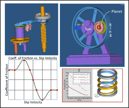
Figure 6 - Examples of contact elements. Both 2-D contact and 3-D contact can be handled by MotionSolve

•

Rigid-flex and flex-flex contact: These are usually modeled as point-to-deformable-curve force elements, point-to-deformable-surface force elements, or deformable-surface-to-deformable-surface force elements. The curve or surface has the ability to deform during the simulation. Figure 7 below shows a spherical body in impact with a highly deformable surface.

point_to_def_surface_ex

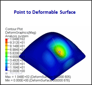
Figure 7 - Point-to-deformable-surface contact force.

•

Abstract system modeling elements: Abstract elements, primarily equations of different kinds are available to represent non-standard components in an MBS model. Differential equations are commonly used to capture the behavior of dynamic subsystems. For instance, these can represent the influence of an air spring in a railway vehicle. Linear and nonlinear state-space equations and transfer functions are also commonly available. These can represent components with well-defined inputs, outputs, and internal states. Figure 8 shows the representation of abstract systems in MotionSolve.

abstract_system_modeling_ms

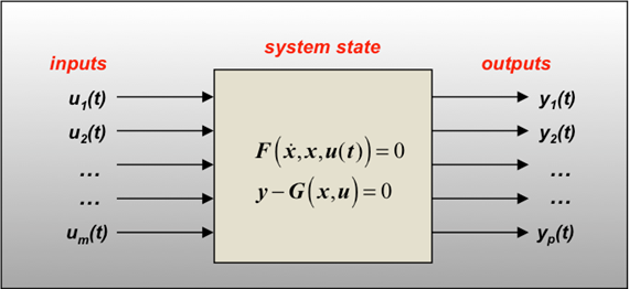
Figure 8 - Abstract system modeling in MotionSolve