The objective of this example is to minimize the volume of a prismatic cantilever beam. The maximum displacement at the beam tip is limited, and the 1st and 2nd eigen frequencies have a lower bound. Two subcases are defined; subcase 1 is the static load case, subcase 2 is the eigenmode analysis.

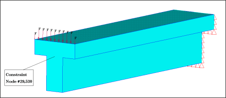
Figure 1: Cantilever beam. Loads and boundary conditions.

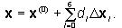
The design domain is subdivided into two design elements; the web and the flange. Six design variables are defined using the design elements and vectors (Fig. 2). For shape optimization, the shape of the beam is defined using the nodal positions of the original shape and a linear combination of the six shape perturbations associated with the design variables. The linear factors are the design variables in the optimization problem. The shape of the beam appears as:

.

Figure 3 shows the shape of the beam perturbed by the first design variable, which is a linear perturbation. Figure 4 shows the quadratic perturbation caused by design variable 4.

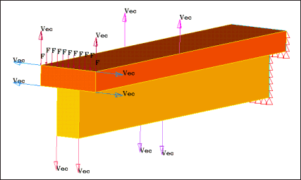
Figure 2: Cantilever beam. Design elements and design variables.

Figure 3: Cantilever beam. Perturbed shape number 1.

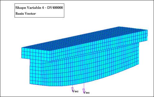
Figure 4: Cantilever beam. Perturbed shape number 4.

The perturbation vectors need to be provided in the format of the DVGRID cards using AutoDV (part of HyperMesh). These cards can be generated automatically. The output of AutoDV also includes the design variable definition DESVAR. The output file Beam_shape.dat can be incorporated into the bulk data section of the OptiStruct input deck via an include statement.

The definition of the optimization problem is included in the case control section of the input deck. Figure 5 shows the section of the OptiStruct input file that includes the definition of the optimization problem and the inclusion of the AutoDV output.

All optimization constraints are met for the model. The final shape is shown in Figure 5.

Cantilever beam. input data
 

$-----------------------------------------------------------------

$

$                      Case Control Cards                                    

$

$-----------------------------------------------------------------

$

DESOBJ(MIN) = 1

$

$HMNAME LOADSTEPS       1Static

$

SUBCASE       1

 LOAD   =    2

 SPC    =    3

 DESSUB =  101

$

$HMNAME LOADSTEPS       2Eigenvalues

$

SUBCASE       2

 SPC    =    3

 METHOD =    4

 DESSUB =        201

$

BEGIN BULK

INCLUDE Beam_shape.dat

$

$  LOAD cards

$

EIGRL, 4, , , 10

$

DRESP1, 1, vol, VOLUME

DRESP1, 2, disp, DISP,,,2,,29530

DCONSTR, 101, 2, -0.01

DRESP1, 3, f1, FREQ,,,1

DRESP1, 4, f2, FREQ,,,2

DCONSTR, 202, 3, 2600.0

DCONSTR, 203, 4, 3000.0

DCONADD, 201, 202, 203

 

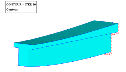
Figure 5: Cantilever beam. Final shape.

For the input file sample, see <install_directory>/demos/hwsolvers/optistruct/beam_shape.fem.

See Also:

Example Problems for Shape Optimization