OS-4020: Composite Bike Frame Optimization

In this tutorial the steps required to perform a ply orientation optimization for a composite structure are covered. The figure below illustrates the model that is used in this tutorial.

4020_frame_model

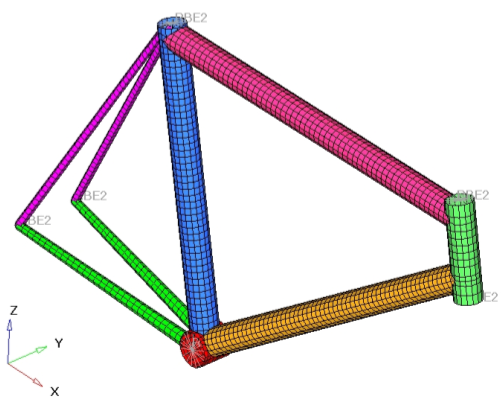
Bicycle frame model

The optimization problem for this tutorial is stated as:

Objective:	Minimize volume.
Constraints:	A given maximum nodal displacement.
Design variables:	Layer thickness.

In this tutorial, you will learn to:

•	Setup the size optimization of a composite bike frame

•	Post-process the composite size optimization results in HyperView

Exercise

Set up the Size Optimization of a Composite Bike Frame

Step 1: Launch the HyperMesh Desktop and Set the User Profile

1.	Launch HyperMesh Desktop.

2.	Choose OptiStruct in the User Profiles dialog and click OK. This loads the user profile. It includes the appropriate template, macro menu, and import reader, paring down the functionality of HyperMesh to what is relevant for generating models for OptiStruct.

3.	Select the Open Model file toolbar icon .

4.	Select the bicycle_frame.hm file you saved to your working directory from the optistruct.zip file. Refer to Accessing the Model Files.

5.	Click Open. The bicycle_frame.hm database is loaded into the current HyperMesh session, replacing any existing data.

The structural model has already been set up with the necessary elements, parts, property, and material data. The next step is to load the frame to simulate a sprint scenario.

Step 2: Create Load Collectors for the Loads and Boundary Conditions

1.	In the Model browser, right-click and click Create > Load Collector.

2.	For Name, enter crank.

3.	Click Color and select any color.

4.	For Card Image, select None.

This creates a new load collector, crank.

5.	Similarly, create another load collector named spcs.

Step 3: Create Loads

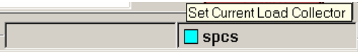
1.	Click Set Current Load Collector at the right bottom corner of the HyperMesh window to enter a new panel in which the load collectors are listed.

4020_set_current_load

2.	Select crank from the list of load collectors.

3.	From the Analysis page, select forces to enter the panel.

4.	Select the create subpanel using the radio buttons on the left-hand side of the panel.

5.	Click the entity selection switch, immediately to the right of the create radio button and select nodes from the pop-up menu.

6.	Select the node at the center of the rigid spider, as seen in the figure below, by clicking on it in the graphical display area.

7.	Set the coordinate system toggle to global system.

8.	Click magnitude = and enter -100.0.

9.	Click the direction definition switch below magnitude = and select the z-axis from the pop-up menu.

10.	Click create. This creates a point force at the pedal location.

11.	Click return to return to the main menu.

12.	From the Analysis page, select the moments panel.

13.	Select the create subpanel using the radio buttons on the left-hand side of the panel.

14.	Click the entity selection switch, immediately to the right of the create radio button and select nodes from the pop-up menu.

15.	Select the node at the center of the rigid spider as seen in the figure below, by clicking on it in the graphical display window.

16.	Set the coordinate system toggle to global system.

17.	Click magnitude = and enter 100.0.

18.	Click the direction definition switch below magnitude = and select the x-axis from the pop-up menu.

19.	Click create. This creates a moment at the pedal location.

4020_loads_applied_lower

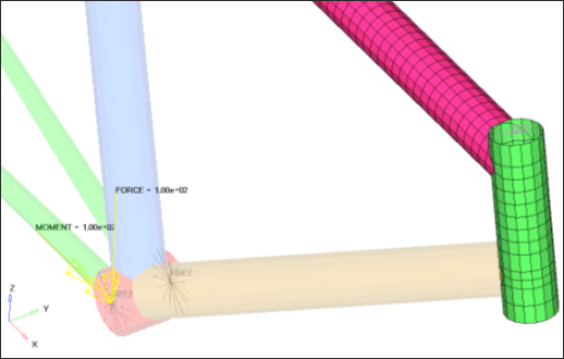
Loads applied to bottom bracket of a bicycle

Note:

This is a simplified loading regime that represents the transformed loads from a person's foot on the pedal.

20.	Click return.

Step 4: Create Constraints

1.	Click Set Current Load Collector at the right bottom corner of HyperMesh window, as in step 3, to enter a new panel in which the load collectors are listed.

2.	Select spcs from the list of load collectors.

Note that spcs now appears on the footer bar to indicate that it is the current load collector.

3.	From the Analysis page, select constraints to enter the panel.

4.	Select the create subpanel using the radio buttons on the left-hand side of the panel.

5.	Click the entity selection switch, immediately to the right of the create radio button and select nodes from the pop-up menu.

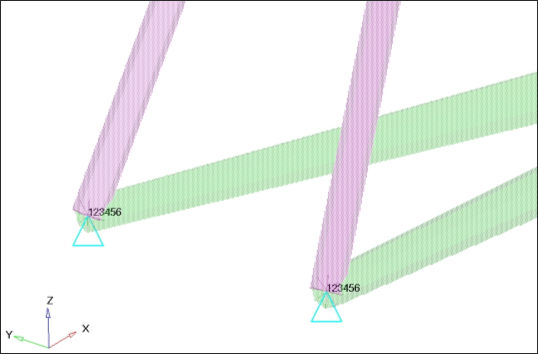
6.	Select the nodes shown below to constrain the structure by clicking on the center of the rigid spiders, as seen in the next two figures.

4020_spcs_to_rear

SPCs applied to rear wheel location of frame

4020_spcs_to_upper

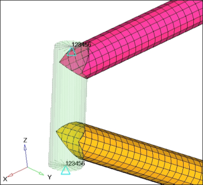
SPCs applied to upper and lower portion of head tube.

7.	Constrain dof1, dof2, dof3, dof4, dof5, and dof6.

Dofs with a check are to be constrained, while dofs without a check will be free.

Dofs 1, 2, and 3 are x, y, and z translation degrees of freedom.

Dofs 4, 5, and 6 are x, y, and z rotational degrees of freedom.

8.	Click create. This applies these constraints to the selected nodes.

9.	Click return to go back to the main menu.

Step 5: Create an OptiStruct Loadstep

1.	In the Model browser, right-click and select Create > Load Step.

2.	For Name, enter crank.

3.	Click Analysis type and select Linear Static from the drop-down menu.

4.	For SPC, click Unspecified > Loadcol.

5.	In the Select Loadcol dialog, select spcs from the list of load collectors and click OK.

6.	For LOAD, click Unspecified > Loadcol.

7.	In the Select Loadcol dialog, select crank from the list of load collectors and click OK.

An OptiStruct loadstep has been created which references the constraints in the load collector spcs and the forces in the load collector crank.

Step 6: Set up the Design Variables

1.	From the 2D page, select the HyperLaminate panel. This launches the HyperLaminate GUI. The next steps are performed in the HyperLaminate GUI.

2.	Expand the Design Variable portion of the tree structure on the left-hand side of the screen. The DESVAR branch appears.

3.	Right-click on DESVAR. A floating menu appears with the option New.

4.	Click New. This creates a new design variable, which is named NewDv1 by default, and the tree structure is expanded.

5.	Rename the design variable to thk1 by right-clicking on NewDv1, select Rename, and overwriting the default design variable name.

6.	In the Initial value: field, enter 1.0.

7.	In the Lower bound: field, enter 0.0.

8.	In the Upper bound: field, enter 2.0.

9.	Click Apply.

10.	In a similar manner, and with identical values, create a total of 5 design variables following the procedure outlined in steps 4 through 9 for thk2, thk3, thk4, and thk5.

Alternately, you can right-click on thk1 and select Duplicate from the floating menu to create an identical design variable. Repeat this process to create a total of 5 design variables, then rename the new design variables by right-clicking on them and selecting Rename.

11.	Examine the PCOMP branch to see all of the PCOMPs in the model.

12.	Select the seat_tube PCOMP. Details of the laminate appear in the GUI.

13.	Click the check box next to Optimization at the top of the middle panel.

New fields appear in the Ply lay-up order table allowing design variables to be associated to ply thicknesses or ply orientations.

14.	Click on the field under Designvar under Optimization in row 1.

15.	Choose thk1 from the drop-down menu.

16.	Repeat steps 14 and 15 for the other rows, as shown below:

4020_designvar

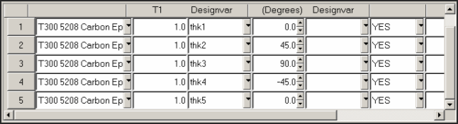
17.	Click Update Laminate.

This associates the design variables thk(i) with the thickness for the ply(i) of this laminate. In this case, ply(11-i) too, since this is a symmetric laminate.

18.	Repeat this process for TOP_tube and down_tube using the same DVs as on the seat_tube property.

19.	Click Exit from the File menu.

Exiting the HyperLaminate GUI and returning to HyperMesh.

Step 7: Create a Displacement and Volume Response

Create a response to measure the total displacement of the node where the loads have been applied and set the objective to minimize this response.

1.	From the Analysis page, select optimization to enter the panel.

2.	Select responses to enter this panel.

3.	Click response= and enter disp.

4.	Click the response type: switch and select static displacement from the pop-up menu.

5.	Click the total disp radio button.

6.	Click nodes and select the node at the bottom bracket where the loads were applied by clicking on it in the graphical display window.

7.	Click create.

8.	Click response= and enter volume.

9.	Click the response type: switch and select volume from the pop-up menu.

10.	Leave total set.

11.	Click create.

12.	Click return to go to the optimization panel.

Step 8: Create Constraints on the Displacement Response

1.	Enter the dconstraints panel.

2.	Click constraint= and enter Disp.

3.	Check the box for upper bound =.

4.	Click upper bound = and enter 1.8.

5.	Click response = and select disp from the list of responses. A loadsteps button appears in the panel.

6.	Click loadsteps.

7.	Check the box next to crank and click select.

8.	Click create.

A constraint is defined on the response disp. It states that any solution (min. volume) needs to have a displacement lower than 1.8 mm to be feasible.

9.	Click return to go to the optimization panel.

Step 9: Define the Objective

1.	Select objective to enter the panel.

2.	Click the left-hand switch and select min.

3.	Click response= and choose volume from the pop-up menu.

4.	Click create.

5.	Click return twice to go to the main menu.

Step 10: Run the Optimization

1.	From the Analysis page, select OptiStruct to enter the panel.

2.	Following the input file: field click save as.

3.	Select the directory where you would like to write the OptiStruct model file and enter the name for the model, bicycle_frameOPT.fem, in the File name: field. The .fem extension is suggested for OptiStruct input decks.

4.	Click Save.

The name and location of the bicycle_frameOPT.fem file displays in the input file: field.

5.	Set the export options: toggle to all.

6.	Set the run options: toggle to optimization.

7.	Set the memory options: toggle to memory default.

8.	Click OptiStruct. This launches the OptiStruct job.

If the job is successful, new results files can be seen in the directory where the OptiStruct model file was written. The bicycle_frameOPT.out file is a good place to look for error messages that will help to debug the input deck if any errors are present.

Post-processing the Composite Size Optimization Results in HyperView

Step 11: Review the Results in HyperGraph

View the design variable and objective history.

1.	Open a session of HyperView using the Add Page icon.

2.	From the File menu, select Open. An Open Session File browser window appears.

3.	Select the bicycle_frameOPT_hist.mvw file that was created from your OptiStruct run and click Open.

This file contains plots of the objective, constraints, and design variables against iteration history. The first page shows the Objective function.

4020_objective_function

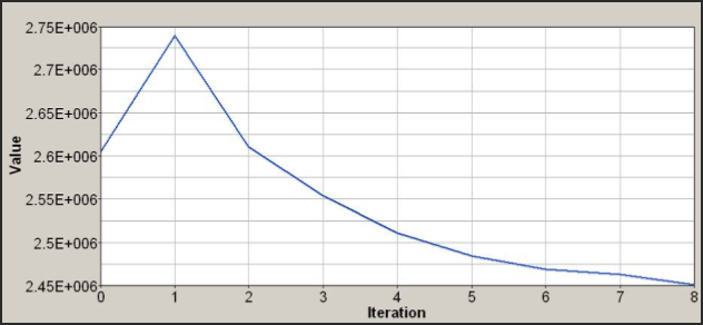
Objective function (Volume) for each iteration.

The second page shows the Maximum Constraint Violation.

4020_iteration

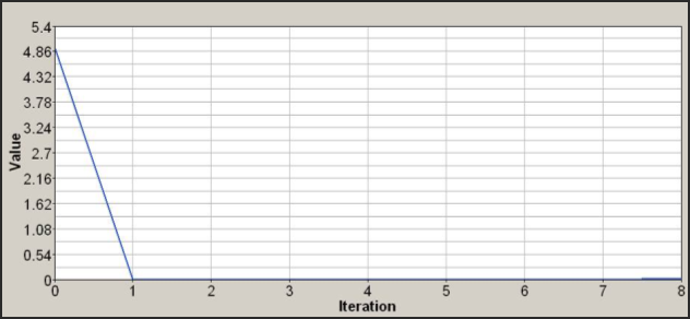
Maximum constraint violation (% [disp > 1.8 mm]) for each iteration.

The next pages show the Design Variables (DVs) which are grouped together making it possible to compare the behavior of the different plies. This plot can be created by opening the bicycle_frameOPT.hgdata file.

4020_dvs

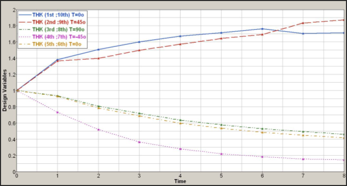
Design variable values for each iteration.