OS-5030: Buckling Optimization of a Structural Rail

Structures are said to "buckle" when a certain combination of loads cause them to be unstable and deflection occurs. When a particular loading is reached, the structure continues to deflect without an increase in the magnitude of the load. The critical load at which buckling occurs is the product of the critical buckling factor and the applied reference load. The buckling factor is an eigenvalue and has no dimension. Generally speaking, the lowest buckling load is usually of the most interest to engineers, since a structure will fail prior to reaching any higher buckling loads.

When using OptiStruct to solve a linear buckling problem, apply a reference load to the structure and calculate the buckling factors based on linear static and normal mode analysis. Use OptiStruct also to perform size and/or shape optimizations on the structure to optimize for linear buckling. Neither yielding of a structure nor change of force can occur during the optimization process.

In this tutorial, a size and shape optimization are performed on a structural rail to increase the buckling factor, thereby increasing the load it can carry before buckling. The rail has external forces applied at one end, and is constrained in all degrees of freedom at the other end. By performing buckling optimization, the buckling factor can be increased and thereby increase critical buckling force.

Buckling optimization needs be performed to minimize the maximum von Mises stress among several elements. This is done using the minimized maximum problem setup. Use MINMAX or MAXMIN statements to define the objective function of a minimize maximum or maximize minimum problem. Many times you will need to minimize or maximize several responses; minimizing the maximum von Mises stress among several elements, for example. In such situations, using user-defined equations to minimize the maximum von Mises stress will not achieve the expected result. Reducing the maximum stress in one element often results in increased stress on another element.

This tutorial describes the steps involved in defining linear buckling and size optimization using the gauge panel. Shape and size optimizations will both be applied to this structural optimization. The shape optimization has been pre-defined in this model using HyperMorph, so you will not need to set up the shapes and shape design variables. The size optimization is part of the exercise. A reference value is given to the stress design objective, and the problem is formulated as a minmax optimization problem. The resulting structure is thicker and wider to prevent buckling.

os5030_pic1

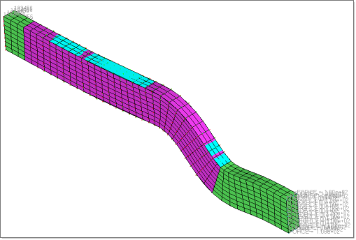
Buckling optimization of a structural rail

Problem Statement

This problem will perform a size and shape optimization on a structural rail to prevent buckling in the rail structure.

Objective function:	Minimize maximum von Mises stress.
Constraints:	1) Increase first buckling factor above 30. 2) Regional volume of designable region is less than 800000.
Design variables:	Element thickness and shape perturbation.

In this tutorial, you will learn to:

•	Setup a buckling optimization simulation

•	Post-process the results with HyperView

Exercise

Step 1: Launch the HyperMesh Desktop, Set the User Profile, and Retrieve the File

1.	Launch HyperMesh Desktop.

2.	Choose OptiStruct in the User Profiles dialog and click OK.

3.	From the File menu on the toolbar, select Open > Model.

4.	Select the os_buckle_original.hm file you saved to your working directory from the optistruct.zip file. Refer to Accessing the Model Files.

5.	Click Open. The os_buckle_original.hm database is loaded into the current HyperMesh session, replacing any existing data.

Setting Up a Buckling Optimization Simulation

Step 2: Review Previously Defined Shape Design Variables and Animation of Shape Changes

The shape optimization is already pre-defined using HyperMorph in this model. You will review the design variables and animation of the previously defined shape changes.

1.	In the Model browser, click the Utility tab.

If the Utility tab is not visible on the left side of the GUI in HyperMesh, go to the View menu, and select Browsers > HyperMesh > Utility.

2.	On the Utility tab, select Opti (near the bottom).

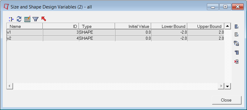
3.	Under Optimization Info:, click Design Variables. The Size and Shape Design Variables dialog appears.

v1 and v2 are pre-defined with Initial Value = 0.0, Lower Bound = -2.0, and Upper Bound = 2.0 (shown below).

5030_dvs

4.	Click Close to close the Size and Shape Design Variables window.

5.	From the Analysis page, click optimization.

6.	Click shape.

7.	Set the radio button to desvar, and click animate.

8.	Set simulation = to SHAPE - v1 (1).

9.	Set data type = to Perturbation Vector.

10.	Click linear and notice the animation of the first shape.

11.	To review the second shape, repeat steps 7 through 9, setting change simulation = to SHAPE - v2 (2).

12.	Click return three times to go back to the Optimization panel.

Step 3: Define the Size Optimization Design Variable

The shape optimization setup is predefined in os_buckle_original.hm. Therefore, you only need to define the size design variable for this buckling optimization problem.

1.	From the Optimization panel, select the gauge panel.

2.	Verify that the create subpanel is selected with the radio buttons on the left.

3.	Set the type: switch to PSHELL-T and the toggle beneath to same desvar for all props.

4.	Click desvar= and enter shells.

5.	Click props.

6.	Click both dom and shell_elements.

7.	Click select.

8.	For initial value =, enter a value of 6.0.

9.	Click the first toggle and change from lower bound % = to lower bound = and enter a value of 3.0.

10.	Click the second toggle and change from upper bound % = to upper bound = and enter a value of 9.0.

11.	Click create.

12.	Click return twice to go back to the main menu.

Step 4: Create Eigenvalue Analysis (buckling) Load Collectors

A load collector to perform real eigenvalue analysis (buckling analysis) will be created.

1.	In the Model browser, right-click and select Create > Load Collector.

2.	For Name, enter Buckling.

3.	Click Color and select any color.

4.	For Card Image, select EIGRL.

5.	Set V1 = 0.01, V2 = 100.0, and ND = 20.

OptiStruct will search for the three lowest eigenvalues below 100.

Step 5: Set up a Buckling Optimization Load Step

1.	In the Model browser, right-click and select Create > Load Step.

2.	For Name, enter Buckling.

3.	Click Color and select a color from the color palette.

4.	Click Analysis type and select Linear buckling from the drop-down menu.

5.	For STATSUB, select the pre-existing LINEAR subcase.

6.	For METHOD(STRUCT), select buckling from the list of load collectors.

Step 6: Define the Responses for Optimization

1.	From the Analysis page, click optimization.

2.	Click responses.

3.	Create three responses with the following settings: Region ID is not required.

Response =	Response type:	Characteristics
Buckle	buckling	Mode Number: 1
Von	static stress	props: dom Stress type: von mises/both surfaces
Vol	volume	by entity props: dom

4.	Click return.

Step 7: Define the Constraints for Optimization

1.	From the optimization panel, click dconstraints.

2.	For constraint =, enter the name BUCKLE.

3.	Click the check box to the left of lower bound and assign a value of 30.

4.	Click response = and click Buckle.

5.	Click loadsteps, then click the box besides the Buckling and click select.

6.	Click create.

7.	Set constraint = VOL and response = Vol.

8.	Uncheck lower bound and click the check box to the left of upper bound to assign a value of 800000.

9.	Click create.

10.	Click return to go back to the Optimization panel.

Step 8: Define the Minimize Maximum Optimization Response

1.	Click obj reference.

2.	For dobjref =, enter the name MAX_STRESS.

3.	Click the check box to the left of pos reference = and enter a value of 1.000.

4.	Click response = and select Von.

5.	Toggle all to loadsteps.

6.	Click loadsteps.

7.	Click the check box to the left of LINEAR, and click select.

8.	Click create. This creates the minimized maximum optimization response.

9.	Click return.

Step 9: Define the Objective for Optimization

1.	Click objective.

2.	Click the switch and set to minmax.

3.	Click dobjrefs.

4.	Check the box to the left of MAX_STRESS.

5.	Click select.

6.	Click create.

7.	Click return twice to go back to the main menu.

Step 10: Solve the Buckling Optimization Problem

1.	From the Analysis page, select the OptiStruct panel.

2.	Click save as.

3.	Select the directory where you would like to write the OptiStruct model file and enter the file name, os_buckle_optimization.fem, in the File name: field. .fem is the suggested extension for OptiStruct input decks.

4.	Click Save.

The name and location of the os_buckle_optimization.fem file displays in the input file: field.

5.	Set the memory options: toggle to memory default.

6.	Click the run options: switch and select optimization.

7.	Set the export options: toggle to all.

8.	Click OptiStruct. This exports the OptiStruct input file and launches the OptiStruct job.

If the job is successful, new results files can be seen in the directory where the OptiStruct model file was written. The os_buckle_optimization.out file is a good place to look for error messages that will help to debug the input deck if any errors are present.

9.	At the end of the optimization run, close the dialog.

Post-processing the Results with HyperView

Step 11: View Animations in HyperView

1.	Click HyperView in the OptiStruct panel.

2.	Close the Message Log window.

3.	Using the page selector arrows (shown below), navigate to the Design History page (page 2).

page_nav

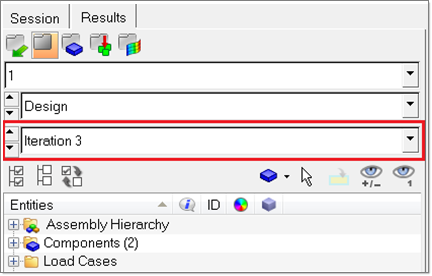
4.	Select Iteration 3 using the drop-down selector in the Model browser, as shown below.

os5030_iteration3

5.	Click the Contour panel toolbar icon .

6.	Under Result type:, select Shape Change (v) from the first drop-down list, and Mag from the second.

7.	Click Apply.

8.	The seek slider and playback speed slider (top and bottom respectively) are located next to the playback controls.

animation_toolbar

9.	With the animation running, use the slider bar to adjust the speed of the animation.

10.	Click the Animation Controls icon next to the seek slider and activate the Bounce option to review a back and forth animation of the impact.

11.	Stop the animation and use the Current time: slider bar to manually control the animation.

For complete details on the various options available in this panel, refer to the online help.

os5030_design_history

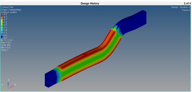
Step 12: View the Stresses on the Final Shape

1.	Click the Next Page arrow to go to the next page (page 3 of 4), which contains the Linear analysis results.

2.	Click the Contour panel toolbar icon.

3.	Under Result type:, select Element Stresses (2D&3D)(t) from the first drop-down list, and vonMises from the second.

4.	Select the final iteration (Iteration 3) using the drop-down selector in the Model browser as shown in step 11.

5.	Click Apply.

A plot of the stresses on your final shape should be displayed.

os5030_linear

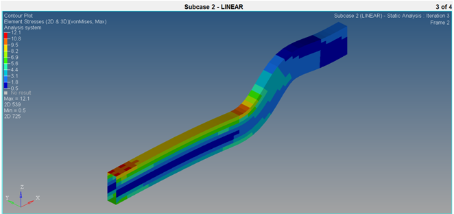
Step 13: View the Buckling Modes

1.	Click the Next Page arrow to go to the next page (page 4 of 4), which contains the buckling results.

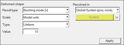
2.	Click the Deformed icon contained within the HyperView toolbar, as shown below. Set the deformed shape parameters to the same as those below. This will improve the animation visualization that will be performed in the next step.

os5030_deform

3.	Select the animation mode toolbar icon and go to Modal.

4.	Click the Animation Controls toolbar icon.

5.	With the animation running, use the speed slider bar to adjust the animation.

Increase the scale to better see the buckling mode shape.

6.	Activate the Bounce option to review animation of the impact.

7.	The animation can also be manually controlled using the time slide to manually control the animation.