Using the MotionSolve API

A. As an alternative to the XML syntax

Any model built using XML syntax can be rewritten in a much more compact and readable way using the MotionSolve Python Interface. The example below illustrates this with a simple model.

from msolve import *

def sliding_block (out_name):

m = Model (output=out_name)

grav = Accgrav (jgrav=-9.800)

dstiff = Integrator (type="DSTIFF", error=1e-5)

p0 = Point (10,0,0)

ux = Vector (1,0,0)

uz = Vector (0,0,1)

grnd = Part (ground=True)

oxyz = Marker (body=grnd, label="Global CS")

# Sliding Block

blk1 = Part (label="Block-1", mass=1, ip=[4.9e-4,4.9e-4,4.9e-4])

blk1.cm = Marker (label="Block-1 CM", body=blk1, qp=p0, zp=p0+ux, xp=p0+uz)

# Trans Joint along Global-X

im1 = Marker (label="Joint-1 I", body=blk1, qp=p0, zp=p0+ux, xp=p0+uz)

jm1 = Marker (label="Joint-1 J", body=grnd, qp=p0, zp=p0+ux, xp=p0+uz)

jnt1 = Joint (label="Joint-1", type="TRANSLATIONAL", i = im1, j = jm1)

# Actuator force

sf1 = Sforce (type="TRANSLATION", actiononly=True, i=im1, j=jm1,

label="Actuation Force-1", function="3*sin(2*pi*time)")

so = Output (reqsave=True)

return m

###############################################################################

model = sliding_block ("One-Sliding-Block")

model.simulate (type="DYNAMICS", end=4, dtout=.01)

The XML syntax will be fully supported and enhanced as needed.

B. As a means to simplify model building

You can tailor the API to suit your modeling style and convenience. Here is an example.

Assume that you want to create a revolute joint simply by specifying the following:

•	The two bodies it connects.

•	The location of the connection point.

•	The joint axis orientation in global space.

You do not want to explicitly create Markers.

You could write a "convenience" function and use it. The process for doing so is illustrated below.

# Create a convenience function first

def RevoluteJoint (ibody, jbody, jname, location=[0,0,0], axis=[0,0,1]):

zpoint = location + axis

im = Marker (body=ibody, label=jname + ”_IM”, qp=location, zp=zpoint)

jm = Marker (body=jbody, label=jname + ”_JM”, qp=location, zp=zpoint)

joint = Joint (type="REVOLUTE", label=jname, i=im, j=jm)

return joint

# Now create a joint

myJoint = RevoluteJoint (Part1, Part2, “myJoint”, location=[23,34,45],

axis=[0. 0.5773503, 0.5773502, 0.5773503]

# Create a second joint

yourJoint = RevoluteJoint (Part3, Part4, “yourJoint”, location=[23,-34,45],

axis=[0. 0.5773503, -0.5773502, 0.5773503]

In a similar manner, you can introduce an entire library of convenience functions and use these to simplify your modeling.

C. Manage user-subroutines

The MotionSolve Python Interface allows you to use user-subroutines in Fortran, C, C++ and Python just as MotionSolve can. However, when the user-subroutine is written in Python, it provides for a very elegant way to resolve path and function name issues.

Consider the following example, where you want to define a rotational SFORCE, but the user subroutine for it, fricTorque(), is defined in a second file. A simple way to handle this is as follows:

# Import the function so Python knows about it

from friction_models import fricTorque

# Define the SFORCE now

sf07 = Sforce (label="sfo7", i=m71, j=m81, type="ROTATION", function=”user(0.2, 0.3, 10)”,

routine=fricTorque)

Python will store the pointer for the function fricTorque with the routine attribute, so path names are easily handled.

D. Create “designable” solver models

Parametric objects and models

Python by itself provides you the ability to create parametric models. Consider the simple example below, where a spherical part is to be created. SI units are used for this example.

•	The material is steel. Its density: rho=7800 Kg/m3

•	The radius of the sphere is: r

•	The mass of the sphere is: m = (4/3) * pi * r3 * rho Kg

•	The inertia of the sphere about is center is: Ixx = Iyy = Izz = ½ * m * r2

You can create a function sphere to create a spherical Part given its density rho, radius r and location loc, as follows:

def sphere (r, rho, loc, label):

mass = (4/3) * math.pi * (r**3) * rho

ixx = iyy = izz = 0.5 * mass * r**2

sphere = Part (mass=mass, ip=[ixx,iyy,izz], label=label)

sphere.cm = Marker (part=sphere, qp=loc, label=label + ”_CM”)

return sphere

Then you can use this function to create a parametric spherical PARTs as follows:

# Steel sphere of radius 0.1 m (10 cm)

r1 = 0.10

rho1 = 7800

loc1 = [0,10,-25]

sph1 = sphere (r1, rho1, loc1, "Steel-Sphere")

# Aluminum sphere of radius 0.05 m (5 cm)

r2 = 0.05

rho2 = 2700

loc2 = [23, 34, 45]

sph2 = sphere (r2, rho2, loc2, "Aluminum-Sphere")

The mass properties of both spheres are now parameterized in terms of their radius and density.

The important point to note is that while Python knows about this parameterization, MotionSolve does not. This is because the mass and inertia expressions are evaluated by Python and resolved into numbers and then provided to MotionSolve.

If you want MotionSolve to know about the parameterization, then you need to create Designable Objects.

Designable objects and models

A designable object is one for which MotionSolve knows the parametric relationships. As a consequence, MotionSolve also knows how to calculate the sensitivity of any system response with respect to the design variables used to parameterize the object.

The sequence of steps required to create designable models and perform sensitivity analysis are as follows:

•	Create Design Variables – this is a new class of objects recently introduced in MotionSolve.

•	Parameterize your model using Design Variables.

•	At the model level, create Response Variables.

•	Perform a simulation with DSA (Design Sensitivity Analysis) turned on.

•	MotionSolve will compute the sensitivity of the Response Variables to a change in the Design Variables. This information is made available to you in a variety of ways.

Design variables

A Design variable (Dv) is an object that contains a label and value. The label is the name of the Dv, and the value is the value of the Dv. Here is an example of a design variable:

bx = Dv ( label="X coordinate of Point B", b=1.0/math.sqrt(2))

You can perform normal mathematical operations with Dvs, just as you can with numbers. Thus:

>>> bx

<msolve.Model.Dv object at 0x0000000001F0B668>

>>> a1 = bx+bx

>>> a1

1.414213562373095 # 1/sqrt(2) + 1/sqrt(2) = sqrt(2) = 1.414213562373095

>>> a3 = bx*bx

>>> a3

0.4999999999999999 # 1/sqrt(2) * 1/sqrt(2) = 1/2

MotionSolve knows variables a1 and a3 are dependent on the Design Variables that bx points to.

So, now you can do parameterization with Design Variables and MotionSolve knows about the parametric relationships. The example below illustrates the creation of parametric spherical PARTS.

Note	You can parameterize the sphere location with design variables also. In the example below, we have not done so.

# Steel sphere of radius 0.1 m (10 cm)

r1 = Dv (label=”Radius of sphere-1”, b=0.10)

rho1 = Dv (label=”Density of Steel”, b=7800)

loc1 = [0,10,-25]

sph1 = sphere (r1, rho1, loc1, "Steel-Sphere")

# Aluminum sphere of radius 0.05 m (5 cm)

r2 = Dv (label=”Radius of sphere-2”, b=0.05)

rho2 = Dv (label=”Density of Aluminum”, b=2700)

loc2 = [23, 34, 45]

sph2 = sphere (r2, rho2, loc2, "Aluminum-Sphere")

MotionSolve knows that the mass and inertias of sph1 are dependent on r1 and rho. Similarly, it knows that the mass and inertias of sph2 are dependent on r2 and rho. Parts sph1 and sph2 are “designable”.

Points and Vectors

Much of the modeling and parameterization in MotionView is done with Points and Vectors. The MotionSolve-Python interface supports Point and Vector classes. These helper classes are provided to simplify MotionSolve models and easily capture MotionView model parameterization in MotionSolve models.

Vector Class

A Vector is an object that has a magnitude and a direction. In this release, vectors are always defined in the global reference frame. They do not rotate or move with any Body in the model.

A Vector is a list of 3 real values. Vector does not accept any other data types. It supports many methods so you can use it in a variety of ways. Here are some built-in methods for Vectors.

Creating a Vector	Create a copy of a Vector	Indexing into a Vector
>>> u=Vector(1,2,3) >>> u Vector (1.0, 2.0, 3.0) >>> v=Vector(-3,0,1) >>> v Vector (-3.0, 0.0, 1.0)	>>> w = u.copy() >>> w Vector (1.0, 2.0, 3.0)	>>> u.x 1 >>> u.y 2 >>> u[2] 3

Unary minus	Addition	Subtraction
>>> -u Vector (-1.0, -2.0, -3.0)	>>> u+v Vector (-2.0, 2.0, 4.0)	>>> u-v Vector (4.0, 2.0, 2.0)

Dot Product of 2 vectors	Cross Product of two vectors	Angle between two vectors
>>> u%v 0 >>> u.dot(v) 0	>>> u*v Vector (0.169030850946, -0.845154254729, 0.507092552837)	>>> u.angle(v) 1.5707963267948966 >>> u.angle(v, degrees=True) 90.0

Magnitude of a vector	Create a unit vector	Scale a vector with a factor
>>> u.magnitude() 3.7416573867739413	>>> u.normalize() Vector (0.267261241912, 0.534522483825, 0.801783725737)	>>> u*10 Vector (10.0, 20.0, 30.0) >>> u.scale(10) Vector (10.0, 20.0, 30.0)

Point Class

A Point is a location in space. It is represented as list of 3 real values. Point does not accept any other data types. The three values are the coordinates of the location in space with respect to some other point. Whenever operations are to be performed with Points, you have to make sure all Point coordinates are expressed in the same coordinate system. Point supports many methods so you can use it in a variety of ways. Here are some built-in methods for Points.

Creating a Point

>>> p=Point(1,2,3)

>>> P

Point (1.0, 2.0, 3.0)

>>> q=Vector(-3,0,1)

>>> v

Point (-3.0, 0.0, 1.0)

Create a copy of a Point

>>> r = p.copy()

>>> r

Point (1.0, 2.0, 3.0)

Indexing into a Point

>>> u.x

>>> u.y

>>> u[2]

Unary minus

>>> -P

Point (-1.0, -2.0, -3.0)

Addition

>>> p+q

Point (-2.0, 2.0, 4.0)

Subtraction

>>> p-q

Point (4.0, 2.0, 2.0)

Distance between 2 points

>>> p.distanceTo(q)

4.898979485566356

>>> q.distanceTo(p)

4.898979485566356

(Distance) Along

>>> p.along(q, 10)

Point (5.08248290464, -2.08248290464, -5.16496580928)

Scaling

>>> p*10

Vector (10.0, 20.0, 30.0)

>>> p.scale(10)

Vector (10.0, 20.0, 30.0

Designable entities using Point and Vector

The location and orientations of Markers can be made functions of points and vectors, and therefore, all connectivity can be made “designable”. The example below illustrates.

>>> #Create a designable Point

>>> px = Dv (b=1)

>>> py = Dv (b=2)

>>> pz = Dv (b=3)

>>> p = Point(px,py,pz)

>>> p

Point (1.0, 2.0, 3.0)

>>> #Create a Part

>>> p2 = Part (mass=1, ip=[1e-4,1e-4,1e-4])

>>> p2.cm = Marker (body=p2)

>>> #Create a designable Marker – its origin and orientation are designable

>>> p2.left = Marker (body=p2, qp=p, zp=p+[0,0,1], label="Left end")

>>> p2.left.qp

Point (1.0, 2.0, 3.0)

Now you can do Design Sensitivity Analysis with these designable MBS entities. The Python Interface has the ability to capture all reasonable MotionView parameterization in a MotionSolve model.

Finally, here is an example that shows how both PARTs and MARKERs can be made designable.

def cyl_mass_prop (l, r, rho):

"""

calculate mass properties of a cylinder, given

(1) length = l

(2) radius = r

(3) density =rho

"""

r2 = r*r

l2 = l*l

mass = math.pi * r2 * l * rho

ixx = iyy = mass * (3 * r2 + l2) / 12

izz = mass * r2 / 2

return mass, ixx, iyy, izz

# Define the design variables (Units are Kg-mm-sec-Newton)

ax = Dv ( label="X coordinate of Point A", b=0)

ay = Dv ( label="Y coordinate of Point A", b=0)

bx = Dv ( label="X coordinate of Point B", b=40)

by = Dv ( label="Y coordinate of Point B", b=200)

rad = Dv ( label="Cylinder radius", b=10)

rho = Dv ( label="Cylinder density", b=7.8E-6)

# Define the points A, B

pa = Point (ax,ay,0) # 0, 0, 0

pb = Point (bx,by,0) # 40, 200, 0

# Link length

lab = pa.distanceTo (pb)

# Crank: cylinder of length lab, radius=rad, density=rho

m2, ixx2, iyy2, izz2 = cyl_mass_prop (lab, rad, rho)

p2 = Part (mass=m2, ip=[ixx2, iyy2, izz2, 0, 0, 0], label="Body Crank")

qploc = (pa+pb)/2

xploc = qploc + [0,0,1]

p2.cm = Marker (body=p2, qp=qploc, zp=pb, xp=xploc, label="Crank cm marker")

In the above example:

•	Part p2 is designable – MotionSolve knows that its mass and inertia are functions of the locations of points A (defined by DVs ax, ay) and B (defined by DVs bx, by), the cylinder radius, rad, and its density, rho.

•	Similarly, the Marker, p2.cm, is designable. It’s location and orientation is dependent on the design variables ax, ay, bx and by.

E. Create your own modeling elements

The MotionSolve Python Interface allows you to create higher level modeling elements and use these. The example below explains in detail. Note, the example shown below could have been done without using the MotionSolve Python Interface, however, it would have been harder to create and more difficult to use.

MotionSolve provides a rich library of general purpose and phenomena specific modeling elements. You can combine these to define new modeling elements that exhibit new behavior. This process is called aggregation. MotionSolve provides a special Composite class to represent such objects.

The Composite Class

Composite is a special class that allows you to aggregate entities, such as Parts, Markers, Forces, Differential Equations, Algebraic Equations and other MotionSolve primitives. A composite class object behaves just like any other solver object except it is a collection of entities conveniently packaged together. They behave as atomic entities and can be instantiated multiple times. The composite class you create is inherited from the built-in Composite class. The examples below shows how you can create your own composite class.

For example, assume you want to create a composite class called a low pass ButterworthFilter. The link explains the Butterworth filter is in great detail – it is summarized here. A low pass filter allows low frequency signals to pass through. It attenuates (decays) high frequency signals. A cutoff frequency defines the frequency at which the attenuation begins. As the frequency increases, the degree of attenuation increases. Butterworth filters have an order; the higher the order the more rapid is the cutoff.

The ButterworthFilter class inherits from the Composite class as shown below.

from msolve import *

class ButterworthFilter (Composite):

Inside this class you can assign properties that you need. In this instance we wish to create a filter having an order in the range 1 ≤ order ≤ 4, with a default order of 3. Of course, you also need an input signal to operate on and an output signal to return the results. So the class with properties is:

from msolve import *

class ButterworthFilter (Composite):

inputSignal = Function()

outputSignal = Function ()

order = Int (3)

You have to write two special methods createChildren and updateChildren to define the behavior of this class. You can also optionally write a validate method, validateSelf.

•

createChildren: Used to create all the MotionSolve entities that are needed by the composite class. When the composite class object is created, the createChildren method is invoked. This happens only once, at the creation of the composite object. In createChildren you will instantiate various MotionSolve objects and define their immutable properties.

•

updateChildren: Used to define all the mutable properties of the class. For instance, the coefficients of the Butterworth filter depend on the order of the filter. Similarly, the input signal to act on can be changed. The updateChildren method defines the order of the filter and the input signal. They can also be defined in the createChildren method – but this is optional.

•	validateSelf: Checks the input to ensure that the data provided to the ButterworthFilter object is physically meaningful.

For the Butterworth filter example, the three methods may look as follows:

from msolve import *

class ButterworthFilter (Composite):

"""The Butterworth filter is a type of signal processing filter designed to have

as flat a frequency response as possible in the passband. It is also referred

to as a maximally flat magnitude filter and it is generally used to eliminate

high frequency content from an input signal.

"""

inputSignal = Function ()

outputSignal = Function ()

order = Int (3)

#- topology ----------------------------------------------------------------

def createChildren (self):

"""This method is called once when the object is created. It is used to

define all the ‘immutable’ properties of the class. The Butterworth

filter consists of the following:

* A string containing the function expression defining the input signal

* A VARIABLE that defines the input signal

* A TFSISO that captures the input to output relationship

* An ARRAY of type ‘X’ to hold the internal states of the TFSISO

* An ARRAY of type ‘Y’ to hold the output from TFSISO

* An ARRAY of type ‘U’ to hold the input signal to the TFSISO

* A string that defines the function expression to access the output

"""

self.var = Variable (function=self.inputSignal)

x = Array (type="X")

y = Array (type="Y")

u = Array (type="U", size=1, variables=[self.var])

num = [1]

den = [1, 2, 2, 1]

self.tf = Tfsiso (label="Butterworth Filter", x=x, y=y, u=u, numerator=num,

denominator=den)

self.outputSignal = "ARYVAL({id},1)".format(id=y.id)

#- Update Children -----------------------------------------------------------

def updateChildren (self):

"""This is called when the property value changes to propagate the change

to the child objects

"""

self.var.function = self.inputSignal

if self.order == 1:

self.tf.denominator = [1, 1]

elif self.order == 2:

self.tf.denominator = [1, math.sqrt(2), 1]

elif self.order == 3:

self.tf.denominator = [1, 2, 2, 1]

elif self.order == 4:

self.tf.denominator = [1, 2.6131, 3.4142, 2.6131, 1]

#- validate ----------------------------------------------------------------

def validateSelf (self, validator):

validator.checkGe ("order", 1)

validator.checkLe ("order", 4)

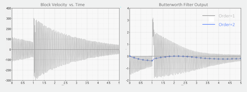
Having created the ButterWorth composite class, you can now use it as an “atomic” object in any model. The example below is a nonlinear mass-spring-damper that oscillates in the global y-direction. Gravity is in the negative y-direction. An impulsive force of 100N is provided in the y-direction at T=1 second. The impulse ends at 1.1 seconds.

Our goal is to pass the velocity of the CM of the mass to the Butterworth filter and obtain a filtered signal as output. The response of the Butterworth filter at order=1 and order=2 are compared.

###############################################################################

## The Model ################################################################

###############################################################################

def butterworthFilter ():

m = Model ()

Units (mass="KILOGRAM", length="MILLIMETER", time="SECOND", force="NEWTON")

Accgrav (jgrav=-9800)

Integrator (error=1e-7)

ground = Part (ground=True)

# Mass

block = Part (mass=1.4702, ip=[44144.717,44144.717,73.5132,0,0,0])

block.cm = Marker (part=block, qp=[0,10,0], zp=[0,11,0])

# Translational joint

jjm = Marker (part=ground, qp=[0,0,0], zp=[0,1,0])

jnt = Joint (type="TRANSLATIONAL", i=block.cm, j=jjm)

# Nonlinear Spring-damper

fexp = "-10*(DY({i},{j})-10)**3 -1e-3*VR({i},{j})".format(i=block.cm.id, j=jjm.id)

nlspdp = Sforce (type="TRANSLATION", i=block.cm, j=jjm, function=fexp)

# Impulse force

iforce = "STEP(TIME, 1, 0, 1.04, 10) * STEP(TIME, 1.05, 10, 1.1, 0)"

sfim = Marker (part=block, qp=[0,10,0], zp=[0,11,0])

impulse = Sforce (type="TRANSLATION", actiononly=True, i=sfim, j=jjm, function=iforce)

# Filter

inputSignal = "VY({i}, {j})".format(i=block.cm.id, j=jjm.id)

m.filt = ButterworthFilter (inputSignal=inputSignal, order=1)

# Requests

m.r1 = Request (type="DISPLACEMENT", i=block.cm, j=jjm)

m.r2 = Request (type="VELOCITY", i=block.cm, j=jjm)

m.r3 = Request (type="ACCELERATION", i=block.cm, j=jjm)

m.r4 = Request (type="FORCE", i=block.cm, j=jjm)

m.r5 = Request (f2=m.filt.inputSignal, f3=m.filt.outputSignal)

m.r6 = Request (type="FORCE", i=sfim, j=jjm)

return m

###############################################################################

## Entry Point ################################################################

###############################################################################

if __name__ == "__main__":

m = butterworthFilter (“butterworth-1”)

m.simulate (type="DYNAMICS", end=5, dtout=0.005)

m.reset()

m = butterworthFilter ("butterworth-2")

m.filt.order = 2

m.simulate (type="DYNAMICS", end=5, dtout=.005)

m.reset()

Due to the action of gravity, the mass sinks down. Since there is a little damping in the system, the systems starts oscillating in the global y-direction with a decaying magnitude. At Time=1 second, the impulse force provides a jolt to the system. The system responds to the jolt and starts settling down again. The model behavior is shown below.

msolve_api_graph1

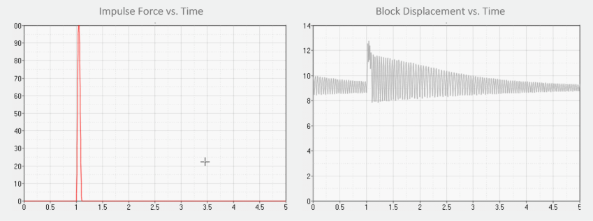
The plot on the left below shows the velocity of the Block as a function of time. This is the input to the transfer function. The plot on the right below shows the response of the order-1 and order-2 Butterworth filters. Notice how the second order filter eliminates the high frequency content.

msolve_api_graph2

DocString

Note that Python has a powerful build in help mechanism that allows to associate documentation with modules, classes and functions. Any of such objects can be documented by adding a string constant as the first statement in the object definition. The docstring should describe what the function or class does. This allows the users and the programmer to inspect objects classes and methods at runtime by invoking the help function on a class, function or object instance.

For example the Butterworth class defined in the example above can be inspected by typing:

help (ButterworthFilter)

Provided that the module has been successfully imported in the current Python namespace, the above command will cause the Python interpreter to output the content of the docstring associated to the ButterworthFilter class. It is generally recommended to add docstrings for all objects, methods and modules in Python. The following snippet shows how module, class, method and function docstrings are defined.

"""

Assuming this is file mymodule.py, then this string, being the

first statement in the file, will become the "mymodule" module's

docstring when the file is imported.

"""

class MyClass(object):

"""The class's docstring"""

def my_method(self):

"""The method's docstring"""

def my_function():

"""The function's docstring"""

Friction modeling example

Friction is a natural phenomenon that occurs in many engineering systems. Friction models contain a variety of nonlinear features such as discontinuities, hysteresis, internal dynamics, and Coulomb friction. These properties cause the friction models to be numerically stiff and computationally cumbersome. The LuGre (Lundt-Grenoble) model for friction is well known in the literature. It is capable of representing several different effects:

•	Dynamic friction

•	Static or Coulomb friction

•	Rate dependent friction phenomena, such as varying breakaway force and frictional lag

The model is defined in terms of the following input parameters:

•	VS = Stiction to dynamic friction transition velocity

•	MUS = Coefficient of static friction

•	MUD = Coefficient of dynamic friction

•	K0 = Bristle stiffness

•	K1 = Bristle damping

•	K2 = viscous coefficient

The friction model is formulated as follows:

•	V = VZ (I, J, J, J) ## Velocity in joint

•	P = -(v/VS)**2 ## Stribeck factor

•	N = sqrt (FX(I, J, J)2 + FY(I,J,J)2) ## The normal force

•	Fc = Mud*N ## Coulomb friction

•	Fs = Mus*N ## Static Friction

•	G = (Fc + (Fs-Fc)*eP)/K0

•	ż = v - \|v\|*z / G ## ODE defining bristle deflection z

•	F = -(K0z + K1zdot + K2*v) ## The friction force

The LuGre friction force consists of 2 atomic elements:

•	A DIFF defining the bristle deflection

•	A FORCE defining the friction element

The composite class can be defined as shown below.

from msolve import *

################################################################################

## LuGre Friction Element ######################################################

################################################################################

class LuGre (Composite):

"""

Create a friction force on a translational joint using the LuGre friction

model.

The LuGre friction force consists of 4 atomic elements:

1. A DIFF defining the bristle deflection

2. A MARKER defining the point of action of the friction force

3. A FORCE defining the friction element

4. A REQUEST capturing the friction force on the block

"""

joint = Reference (Joint)

vs = Double (1.E-3)

mus = Double (0.3)

mud = Double (0.2)

k0 = Double (1e5)

k1 = Double (math.sqrt(1e5))

k2 = Double (0.4)

#- topology ----------------------------------------------------------------

def createChildren (self):

"""This is called when the object is created so the children objects

"""

# The DIFF defining bristle deflection

self.diff = Diff (routine=self.lugre_diff, ic=[0,0])

# The MARKER on which the friction force acts

self.im = Marker ()

# The FORCE defining the friction force

self.friction = Sforce (type="TRANSLATION", actiononly=True,

routine=self.lugre_force)

# The REQUEST capturing the friction force

self.request = Request (type="FORCE", comment="Friction force")

#- Update Children -----------------------------------------------------------

def updateChildren (self):

"""This is called when the property value changes to propagate the change

to the child objects

"""

self.friction.i = self.joint.i

self.friction.j = self.joint.j

self.im.setValues (body=self.joint.i.body, qp=self.joint.i.qp, zp=self.joint.i.zp)

self.request.setValues (i=self.im, j=self.joint.j, rm=self.joint.j)

#- validate ----------------------------------------------------------------

def validateSelf (self, validator):

validator.checkGe0 ("VS")

validator.checkGe0 ("MUS")

validator.checkGe0 ("MUD")

validator.checkGe0 ("K0")

validator.checkGe0 ("K1")

validator.checkGe0 ("K2")

if self.mud > self.mus:

msg = tr("Mu dynamic({0}) must be <= Mu static ({1})",

self.mud, self.mus)

validator.sendError(msg)

#- Lugre Diff ------------------------------------------------------------

def lugre_diff (self, id, time, par, npar, dflag, iflag):

"Diff user function"

i = self.joint.i

j = self.joint.j

vs = self.vs

mus = self.mus

mud = self.mud

k0 = self.k0

z = DIF(self)

v = VZ(i,j,j,j)

N = math.sqrt (FX(i,j,j)**2 + FY(i,j,j)**2)

fs = mus*N

fc = mud*N

p = -(v/vs)**2

g = (fc + (fs - fc) * math.exp(p))/k0

if iflag or math.fabs(g) <1e-8:

return v

else:

return v - math.fabs(v) * z / g

#- friction_force -----------------------------------------------------------

def lugre_force (self, id, time, par, npar, dflag, iflag):

"Friction Force user function"

i = self.joint.i

j = self.joint.j

diff = self.diff

k0 = self.k0

k1 = self.k1

k2 = self.k2

v = VZ (i,j,j,j)

z = DIF (diff)

zdot = DIF1 (diff)

F = k0*z + k1*zdot + k2*v

return -F

F. Build models easily with your own modeling elements

A block sliding in a translational joint is used to illustrate how classes you created can be used in simplifying modeling. Notice that the syntax for built-in classes is identical to the syntax for user-created classes.

################################################################################

# Model definition #

################################################################################

def sliding_block ():

"""Test case for the LuGre friction model

Slide a block across a surface.

The block is attached to ground with a translational joint that has

LuGre friction

"""

model = Model ()

Units (mass="KILOGRAM", length="METER", time="SECOND", force="NEWTON")

Accgrav (jgrav=-9.800)

Integrator (error=1e-5)

Output (reqsave=True)

# Location for Part cm and markers used for the joint markers

qp = Point (10,0,0)

xp = Point (10,1,0)

zp = Point (11,0,0)

ground = Part (ground=True)

ground.jm = Marker (part=ground, qp=qp, zp=zp, xp=xp, label="Joint Marker")

block = Part (mass=1, ip=[1e3,1e3,1e3], label="Block")

block.cm = Marker (part=block, qp=qp, zp=zp, xp=xp, label="Block CM")

# Attach the block to ground

joint = Joint (type="TRANSLATIONAL", i=block.cm, j=ground.jm)

# Apply the LuGre friction to the joint

model.lugre = LuGre (joint=joint)

# Push the block

Sforce (type="TRANSLATION", actiononly=True, i=block.cm, j=ground.jm,

function="3*sin(2*pi*time)", label="Actuation Force")

# Request the DISPLACEMENT, VELOCITY and FORCE of the Joint

model.r1 = Request (type="DISPLACEMENT", i=block.cm, j=ground.jm, rm=ground.jm,

comment="Joint displacement")

model.r2 = Request (type="VELOCITY", i=block.cm, j=ground.jm, rm=ground.jm,

comment="Joint velocity")

model.r3 = Request (type="FORCE", i=block.cm, j=ground.jm, rm= ground.jm,

comment ="Joint force")

return model

###############################################################################

## Entry Point ################################################################

###############################################################################

if __name__ == "__main__":

model = sliding_block()

model.simulate (type="DYNAMICS", end=4, dtout=.01)

# Change the static friction coefficient and continue simulation

model.lugre.mus=0.5

model.simulate (type="DYNAMICS", end=8, dtout=.01)

G. Custom simulations

A Simple Example

Just as you can create higher level modeling elements and simplify the task of model building, you can choreograph complex simulations by building your own functions or objects to do so. The previous example shows two sequential simulations being performed.

You can create your own function and invoke this at run time as the example below shows.

# Create a model

m = sliding_block("lugre1")

# Define a custom simulation function

def mySlidingBlockSimulation (m):

m.simulate (type="DYNAMICS", end=4, dtout=.01)

m.lugre.mus=0.5

m.simulate (type="DYNAMICS", end=8, dtout=.01)

# Perform a custom simulation on the model

mySlidingBlockSimulation (m)

The Model object facilitates more complex custom simulation scenarios. This is explained below.

Complex Simulations with The Model Object

def sliding_block (out_name):

Line 6: m = Model (output=out_name)

In the line 6 of the example in Section F, the function sliding_block(), creates a Model object, m. The Model object is a container that stores the entire model. The Model object has several methods that can operate on its contents.

•	sendToSolver – Send the model to the Solver

•	simulate – Perform a simulation on the model

•	save – Store the model and simulation conditions to disk

•	reload – Reload a saved model

•	control – Execute a CONSUB

•	reset – Reset a simulation so the next simulation starts at T=0

You can handle fairly complex simulations using the Model methods on the Model object.

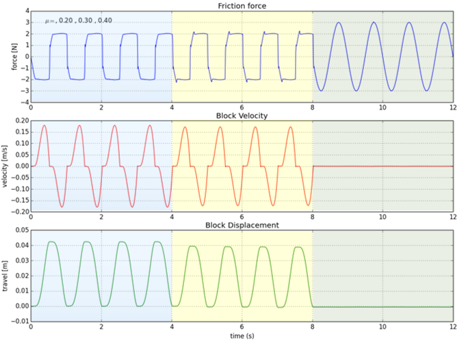
Here is an extension to the simulation script shown earlier.

•	It asks you to specify a μstatic (coefficient of static friction) for the LuGre friction element.

•	It applies this value and performs a simulation.

•	The process repeats and you can continue providing new values of μstatic.

•	The process stops when you issue a STOP command.

•	The script then plots some key results for the various values of μstatic you provided and ends the execution.

The simulation script is shown below.

# Initialize a few variables: duration for each simulation, # simulations done, a string

dur = 4.0

num_simulations = 0

textstr = '$\mu=$'

# Read the model

m = sliding_block()

###############################################################################

# Loop until user asks you to stop #

###############################################################################

while True:

# Get a value for mu static or a command to stop

mus = raw_input (“Please enter a value for mu static or stop: “)

if mus.lower ().startswith ("s"):

break

else:

num_simulations +=1

# Apply the value of mu static the user provided and do a simulation

m.lugre.mus=mus

run = m.simulate (type="DYNAMICS", returnResults=True, duration=dur, dtout=0.01)

textstr += ', %.2f '%(m.lugre.mus)

# Get the request time history from the run object

disp = run.getObject (m.r1)

velo = run.getObject (m.r3)

force = run.getObject (m.r2)

###############################################################################

# Plot some interesting results #

###############################################################################

import matplotlib.pyplot as plt

# Friction force vs. Time

plt.subplot (3, 1, 1)

plt.plot (force.times, force.getComponent (3))

plt.title ('Friction force')

plt.ylabel ('force [N]')

plt.text (0.4, 3, textstr)

plt.grid (True)

# Block Velocity vs. Time

plt.subplot (3, 1, 2)

plt.plot (velo.times, velo.getComponent (3), 'r')

plt.title ('Block Velocity')

plt.ylabel ('velocity [m/s]')

plt.grid (True)

# Block Displacement vs. Time

plt.subplot (3, 1, 3)

plt.plot (disp.times, disp.getComponent (3), 'g')

plt.title ('Block Displacement')

plt.xlabel ('time (s)')

plt.ylabel ('travel [m]')

plt.grid (True)

plt.show()

The results of this simulation are shown below.

msolve_api_graph3

H. Automated ID management

The MotionSolve Python Interface is capable of managing IDs for you. You do not need to specify an ID while you are modeling. However, you can create entities with IDs if you want to. Here is an example.

# Create a RIGID BODY WITHOUT an ID

blk2 = Part (label="Block-2", mass=2, ip=[9.8e-4,9.8e-4,9.8e-4])

# Create a RIGID BODY WITH an ID

blk3 = Part (id=30101011, label="Block-3", mass=2, ip=[9.8e-4,9.8e-4,9.8e-4])

The ID of any object (that can have an ID), can be obtained by using the id attribute of the object. Here are two examples:

>>> blk2.id

>>> blk3.id

30101011

IDs are used in only one place in the MotionSolve Python Interface – for creating function expressions that MotionSolve will evaluate at run time. You can use standard Python programming to construct function expressions. Here is an example that illustrates how you can do this.

Assume that you created a block on a translational joint as shown below.

p0 = Point (10,0,0)

ux = Vector (0,0,1)

ux = Vector (1,0,0)

blk = Part (mass=1, ip=[4.9e-4,4.9e-4,4.9e-4], label="Block")

blk.cm = Marker (body=blk, qp=p0, zp=p0+uz, xp=p0+ux, label="Block CM")

im = Marker (body=blk, qp=p0, zp=p0+ux, xp=p0+uz, label="Joint Marker on Block")

jm = Marker (body=grnd, qp=p0, zp=p0+ux, xp=p0+uz, label="Joint Marker on Ground")

jnt = Joint (type="TRANSLATIONAL", i = im, j = jm, label="Trans Joint")

Now you wish to create a Request that can compute the kinetic energy of the block. Here is how you would do it.

KE = "0.5 * {m} * (VM({blkcm})**2)".format(m=blk.mass, blkcm=blk.cm.id)

r1 = Request (type="EXPRESSION", f2=KE, comment="Kinetic Energy of Block")

I. Easily convert non-designable models to designable models

It is quite straightforward to convert non-designable parametric models into designable models. The example below shows how. The highlighted sections are the changes you need to make to convert a non-designable model (left) to a designable model (right). Essentially, all you need to do is to redefine model parameters of interest to be design variables.

Non-Designable but Parametric Model

Designable Model

ax = 0

ay = 0

bx = 40

by = 200

ax = Dv (b=0, label=”ax”)

ay = Dv (b=0, label=”ay”)

bx = Dv (b=40, label=”bx”)

by = Dv (b=200, label=”by”)

# Define the points A, B

pa = Point (ax,ay,0)

pb = Point (bx,by,0)

# Revolute joint at A

zploc = pa + [0,0,1]

p1.A = Marker (body=p1, qp=pa, zp=zploc)

p2.A = Marker (body=p2, qp=pa, zp=zploc)

ja = Joint (type="REVOLUTE", i=p2.A, j=p1.A)

# spherical joint at B

p2.B = Marker (body=p2, qp=pb)

p3.B = Marker (body=p3, qp=pb)

jb = Joint (type="SPHERICAL", i=p3.B, j=p2.B)

# Define the points A, B

pa = Point (ax,ay,0)

pb = Point (bx,by,0)

# Revolute joint at A

zploc = pa + [0,0,1]

p1.A = Marker (body=p1, qp=pa, zp=zploc)

p2.A = Marker (body=p2, qp=pa, zp=zploc)

ja = Joint (type="REVOLUTE", i=p2.A, j=p1.A)

# spherical joint at B

p2.B = Marker (body=p2, qp=pb)

p3.B = Marker (body=p3, qp=pb)

jb = Joint (type="SPHERICAL", i=p3.B, j=p2.B)

J. Perform Design Sensitivity Analysis

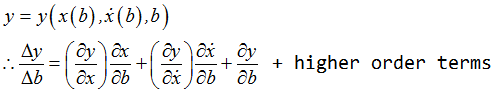
The sensitivity of an output y(u) to an input u is defined as the change in y due to a unit change in u.

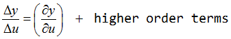
The quantity is called the first order sensitivity of the quantity y to the input u.

Sensitivity analysis is the study of how the change or uncertainty in the output of a mathematical model or system (y) can be apportioned to different sources of change or uncertainty in its inputs (u).

For Design Sensitivity Analysis, the quantity u is not an input, but the design b. Here we are asking the question: For a given change in the design b, how does the response y change.

In a multibody simulation, the response is typically a function of the system states and , and, perhaps, explicitly on the design b. The system states consist of (a) Displacements, (b) Velocities, (c) Lagrange Multipliers (or constraint reaction forces), (d) User defined differential equations, (e) User defined algebraic equations originating from Variables and LSE/GSE/TFSISO outputs, and, (f) Internally created intermediate states that simplify computation. The system states, (the system response), is implicitly dependent on b. Thus .

In mathematical terms:

The equations of motion provide an implicit relationship between (x and b) and (and (x, b)). The quantities 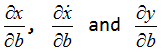need to be computed first. Once these are known, the design sensitivity, , can be computed.

The calculation of is called DSA (Design Sensitivity Analysis) in MotionSolve. This is a new analysis method in MotionSolve. It always accompanies a regular analysis, such as static analysis, quasi-static analysis, kinematic analysis, dynamic analysis or linear analysis. The job of the regular analysis is to compute the states z, ż and the outputs y for a given design b. Once these are known, the DSA analysis will compute the sensitivity, . When there are Ny responses and Nb design variables, is a matrix of dimension Ny x Nb.

There are three well-known methods for computing design sensitivity. These are briefly discussed below.

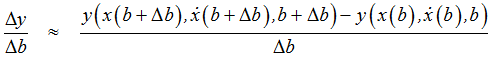
Finite Differencing

As the name implies, this approach uses finite differencing to compute . First, a change in , is selected. Then the change in the output, is computed as shown below.

This is the approach used by HyperStudy, and it can only be used for small-scale design sensitivity analysis (usually 20-30 variables). For a system with Nb design variables, this approach requires simulations. One simulation is required to compute 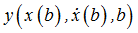. Nb simulations are required to compute , in other words, once for each design variable.

The major issue with this approach is selecting the right . If this is too small, the sensitivities get lost in the numerical error in the solution. If these are too large, the non-linearity of the solution is overlooked. The perturbation is also dependent on the scale and units of the system. In summary, this approach is applicable only for small problems and there are some unresolvable issues about what the perturbations should be.

Direct Differentiation

In this approach, the equations of motion are analytically differentiated with respect to each design variable bi, i=1… Nb. At each point in time, after an analysis step is complete, Nb sets of DAE are solved numerically to yield the required values . This approach is quite robust and is used when the numbers of design variables Nb are not too large. As the number of design variables increase, the cost of the solution also increases.

Adjoint Approach

This is also an analytical approach where finite differencing is not used. The cost of this method, however, is proportional to the number of response variables in the model. The number of design variables does not govern the cost. This approach is quite robust and is used when the numbers of design variables Nb are large.

The example below illustrates how DSA may be performed using the MotionSolve Python Interface. The dsa=“AUTO” setting will select the best approach based on the problem characteristics.

if __name__ == "__main__":

m = sliding_block("lugre1")

m.simulate (type=" STATIC ", dsa=”AUTO”, end=4, dtout=.01)

m.lugre.mus=0.5

m.simulate (type="STATIC", dsa=”AUTO”, end=8, dtout=.01)

At this time, MotionSolve supports DSA only for Kinematic, Static and Quasi-static analyses. DSA is not supported for Dynamic or Linear analyses.

Note also, that in order to compute the sensitivities, MotionSolve needs to know what the design variables are, how the model is parameterized with these design variables and what the response variables are. DSA will yield correct answers only when the model is "designable”. For non-designable models, it will return ZERO as the answer.

K. Perform design optimization

The goal of an optimization run is to minimize an objective function, , specified in the following integral form:

represents the initial value of that may be accumulated from prior analysis when multiple simulates are involved.

You can differentiate the above equation with respect to time, to obtain the following equivalent relationships:

In MotionSolve, the equations are defined through a new modeling element, RV. RV accepts a function expression as input. An initial condition is also specified. As output, it returns the time integral of the expression . RVAL is the output mentioned earlier.

When a DSA is performed, MotionSolve computes the partial derivatives of the RVALs with respect to each of the design variables. This is returned in an array DSARY.

The sensitivity of the cost function, , is in terms of the DSARY.

The Python interface to MotionSolve supports several optimization functions. It is designed to follow a well-defined sequence of steps and require minimal input from you.

The Key Steps to Performing an Optimization:

•	Create a designable model of a system using this interface

•	Instrument the model to be optimization ready

•	Create model responses that you wish to optimize. These are called metrics.

•	Define target values you want for the metrics you defined

•	Create an objective from the metric functions and target values

•	Create an optimizer and give it the objective you defined

•	Ask the optimizer to optimize the system

Example

Select a system to be optimized and create a designable model using this interface

A designable 4-bar mechanism is used for this example.

################################################################################

# Model definition #

################################################################################

def fourbar (design):

"""

The 4 bar is defined with 4 design points A, B, C, D.

coupler (p3)

The 4 bar is an RSUR mechanism B o- - - - - - -o C

R is at Point A / \

S is at Point B ^ Yg / crank \follower

U is at Point C | / \

R is at point D o--->Xg A o~~~~~~~~~~~~~~~~~~~~~o D

The two revolute joints at A and D are defined with their Z-axes along the global Z

The spherical joint at B does not care about orientations

The universal joint at C is defined as follows:

1st z-axis, zi, along global Z

2nd z-axis, zj, perpendicular to zi and the line from B to C

A = (0,0) B=(40,200) C=(360,600) D=(400,0)

The entire model is parameterized in terms of these 4 design points: A, B, C and D.

Since we are operating in 2D space, this leads to 8 DVs: ax, ay, bx, by, cx, cy, dx & dy.

"""

# Helper function to create a PART, MARKERS, GRAPHIC, REQUEST

def make_cylinder (a, b, r, rho, label, oxyz):

""" Create a cylinder, its CM and graphic given:

- End points a and b

- Radius r

- density rho

"""

r2 = r*r

h2 = (a[0]-b[0])**2 + (a[1]-b[1])**2 + (a[2]-b[2])**2

h = math.sqrt(h2)

mass = math.pi * r2 * h * rho

ixx = iyy = mass * (3 * r2 + h2) / 12

izz = mass * r2 / 2

qploc = (a + b)/2

xploc = qploc + [0,0,1]

# Create a PART, its CM, a MARKER for CYLINDER reference, a CYLINDER and a REQUEST

cyl = Part (mass=mass, ip=[ixx, iyy, izz, 0, 0, 0], label=label)

cyl.cm = Marker (body=cyl, qp=qploc, zp=b, xp=xploc, label=label + "_CM")

cyl.gcm = Marker (body=cyl, qp=a, zp=b, xp=xploc, label=label + "_Cylinder")

cyl.gra = Graphics (type="CYLINDER", cm=cyl.gcm, radius=r, length=h, seg=40)

cyl.req = Request (type="DISPLACEMENT", i=cyl.cm, comment=label + " CM displacement")

return cyl

# Create a REVOLUTE or SPHERICAL joint

def make_joint (p1, p2, loc, type):

xploc = loc + [1,0,0]

zploc = loc + [0,0,1]

p1m = Marker (body=p1, qp=loc, zp=zploc, xp=xploc)

p2m = Marker (body=p2, qp=loc, zp=zploc, xp=xploc)

joint = Joint (type=type, i=p1m, j=p2m)

return joint

model = Model (output="test")

units = Units (mass="KILOGRAM", length="MILLIMETER", time="SECOND", force="NEWTON")

grav = Accgrav (jgrav=-9800)

output = Output (reqsave=True)

# define the design variables

ax = Dv ( label="X coordinate of Point A", b=design["ax"])

ay = Dv ( label="Y coordinate of Point A", b=design["ay"])

bx = Dv ( label="X coordinate of Point B", b=design["bx"])

by = Dv ( label="Y coordinate of Point B", b=design["by"])

cx = Dv ( label="X coordinate of Point C", b=design["cx"])

cy = Dv ( label="Y coordinate of Point C", b=design["cy"])

dx = Dv ( label="X coordinate of Point D", b=design["dx"])

dy = Dv ( label="Y coordinate of Point D", b=design["dy"])

kt, ct, rad, rho = 10, 1, 10, 7.8e-6

ux, uz = Vector(1,0,0), Vector(0,0,1) # Global X, # Global Z

pa = Point (ax,ay,0)

pb = Point (bx,by,0)

pc = Point (cx,cy,0)

pd = Point (dx,dy,0)

#Ground

p0 = Part (ground=True)

oxyz = Marker (body=p0, label="Global CS")

#Dummy Part

p1 = Part (label="dummy part")

fj = Joint (i = Marker(body=p0), j = Marker(body=p1), type="FIXED")

#crank, coupler, follower parts

p2 = make_cylinder (pa, pb, rad, rho, "Crank")

p3 = make_cylinder (pb, pc, rad, rho, "Coupler")

p4 = make_cylinder (pc, pd, rad, rho, "Follower")

#revolute joint at A, D & spherical at C

ja = make_joint (p2, p1, pa, "REVOLUTE")

jb = make_joint (p3, p2, pb, "SPHERICAL")

jd = make_joint (p1, p4, pd, "REVOLUTE")

#motion to drive system @A

j1mot = Motion (joint=ja, jtype="ROTATION", dtype="DISPLACEMENT", function="360d*time")

#universal joint at C

xiloc = pc + ux # Xi along global X

ziloc = pc + uz # Zi along global Z

xjloc = pc + uz # Xj along global Z

zixbc = uz.cross (pc-pb).normalize () # unit vector orthogonal to Zi and BC

zjloc = pc+zixbc # Zj of universal joint

p3C = Marker (body=p3, qp=pc, zp=zjloc, xp=xjloc, label="p3C")

p4C = Marker (body=p4, qp=pc, zp=ziloc, xp=xiloc, label="p4C")

jc = Joint (type="UNIVERSAL", i=p4C, j=p3C)

return model

Instrument the model to be optimization ready

We want the x-coordinate of the Coupler CM origin to follow a certain path in the X-Y plane.

•	Define the metric, the expression defining the x-coordinate of the Coupler CM.

•	Define its target value.

# Define the “metric” that is to be optimized

expr = "DX({cm})".format(cm=p3.cm.id)

metric = Variable (label="Coupler DX", function=expr)

# Define the target behavior

splineInput = Variable (label="Spline Independent Variable", function="time")

xval = [0.0, 0.1, 0.2, 0.3, 0.4, 0.5, 0.6, 0.7, 0.8, 0.9, 1.0,

1.1, 1.2, 1.3, 1.4, 1.5, 1.6, 1.7, 1.8, 1.9, 2.0]

yval = [201.0000, 78.0588, -35.2336, -102.143, -112.562, -78.7180, -23.9943, 36.8618,

157.3920, 260.2130, 199.9970, 78.0583, -35.2340, -102.143, -112.562, -78.7178,

-23.9940, 36.8621, 157.3920, 260.2130, 199.9990]

target = Spline (label="Coupler_DX-Target", x=xval, y=yval)

Create an objective from the metric function and target values

# Define the cost function

rmsError = RMS_Relative(signal=splineInput, target=target, metric=metric)

rmsError.setup()

Create an optimizer and give it the objective you defined

# Define the initial design

startDesign = OrderedDict ()

startDesign["ax"] = -15

startDesign["ay"] = 15

startDesign["bx"] = 45

startDesign["by"] = 220

startDesign["cx"] = 345

startDesign["cy"] = 585

startDesign["dx"] = 415

startDesign["dy"] = -15

Create an optimizer

opt = Optimizer (label="Optimize RMS Error", design=startDesign, modelGenerator=fourbar,

objective=rmsError, simType="STATICS", simTend=4.0, simDTout=0.01)

Ask the optimizer to find a final design that will optimize the system

result = opt.optimize (maxit=100, accuracy=1.0e-2)

Examine the result

# Was the optimization successful?

>>> result.success

True

# How many iterations did the optimizer take?

>>> result.nit

# What was the final design?

>>> result.x

[0.01983578586441092, -0.00898945915748043, 39.99727645800783, 199.9829124541905,

359.9752404909047, 600.0265028357005, 399.9737539465066, -0.0009001577101342088]

The exact answer is:

exactX = [0, 0, 40, 200, 360, 600, 400, 0]

The L2 norm of the distance between the results.x and exactX is 0.052714038720902294.

You can see that the optimizer did indeed find an optimal solution.

If you set the accuracy to 1e-3 and rerun, after 26 iterations you will obtain:

>>> result2 = opt.optimize (maxit=100, accuracy=1.0e-3)

>>> result2.x

[-0.00228784659143783, 0.013354616280974424, 40.00015734224888, 200.0138744649529, 359.99195451559245, 599.9837146566314, 400.0200018558606, -0.036468425275888644]

The L2 norm of the distance between the results2.x and exactX is 0.04935654019790089.

You can see that the optimizer did indeed find a better solution, though at the expense of more iterations.

Using the MotionSolve API

Using the MotionSolve API

Using the MotionSolve API

B. As a means to simplify model building

C. Manage user-subroutines

D. Create “designable” solver models

Parametric objects and models

Designable objects and models

Design variables

Points and Vectors

Creating a Vector

Create a copy of a Vector

Indexing into a Vector

Unary minus

Addition

Subtraction

Dot Product of 2 vectors

Cross Product of two vectors

Angle between two vectors

Magnitude of a vector

Create a unit vector

Scale a vector with a factor

Designable entities using Point and Vector

E. Create your own modeling elements

The Composite Class

DocString

Friction modeling example

F. Build models easily with your own modeling elements

G. Custom simulations

A Simple Example

Complex Simulations with The Model Object

H. Automated ID management

I. Easily convert non-designable models to designable models

J. Perform Design Sensitivity Analysis

Finite Differencing

Direct Differentiation

Adjoint Approach

K. Perform design optimization

The Key Steps to Performing an Optimization:

Example

Select a system to be optimized and create a designable model using this interface

Instrument the model to be optimization ready

Create an objective from the metric function and target values

Create an optimizer and give it the objective you defined

Ask the optimizer to find a final design that will optimize the system

Examine the result