The MIT's three Bushing Static Stiffness models include:
The bushing stiffness properties are approximated by a single coefficient–the stiffness at the operating point. The force generated by the bushing is:
F=-k*x
Where:
k
|
is the stiffness.
|
x
|
is the deflection.
|
|
The bushing stiffness is approximated by two cubic polynomials that are derived from the Static Force vs. Deflection curve. Below, the measured static data is shown as a blue curve:
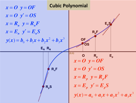
The five points in the selected area of the plot above are:
Point
|
Description
|
Location on Plot
|
O
|
Operating point.
|
The force value, OF, and the slope of the static curve, OS, are selected.
|
Ep
|
End point for positive deformation.
|
This is usually the maximum positive deformation in the static test. At EP, the slope of the static curve, EPS, is selected.
|
Rp
|
Reference point for positive deformation.
|
As a default, RP = (O + EP)/2. At RP, the force of the static curve, RPF, is selected.
|
EN
|
End point for negative deformation.
|
This is usually the maximum negative deformation in the static test. At EN, the slope of the static curve, ENS, is selected.
|
RN
|
Reference point for negative deformation.
|
As a default, RN = (O + EN)/2. At RN, the force of the static curve, RNF, is selected.
|
|
Spline data is derived by reducing the static data to a curve. A cubic spline is fitted through the measured static data. The spline is then used as the interpolating function for calculating the force at any deflection.
|


