This section defines and provides examples of the Sprague-Geers Metric for Data Similarity.
Definition
Consider two signals a(xk) and b(xk), k=1…N. You are interested in computing a metric that shows the similarity of these signals. Use the following steps to compute the Sprague-Geers metric:
| 1. | Calculate the metric M for magnitude difference and P for phase difference as follows: |
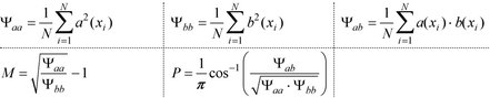
(Click to enlarge)
| 2. | Calculate the combined metric C as follows: |
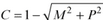
C=1 is a perfect match. Metric C is what we want to show.
| Note: |  is known as the Sprague-Geers Combined Metric. is known as the Sprague-Geers Combined Metric. |
|
Examples
This section provides four plots showing the Sprague-Geers Metric:
Example 1: Signals with the same overall magnitude, but drastically different slopes
Ψaa= 143.50, Ψbb= 143.50, Ψab= 77.00, M=0.00, P=0.319714, C=0.680286
Example 2: Two very similar signals displaced in the y direction by 5%
Ψaa= 0.50, Ψbb= 0.51, Ψab= 0.50, M=-0.009852, P=0.044719, C=0.954208
Example 3: A synthesized MIT example for Dynamic Stiffness
Ψaa= 3.39E+5, Ψbb= 3.77E+5, Ψab= 3.57E+5, M=-0.051164, P=0.026831, C=0.942227
Example 4: A synthesized MIT example for Loss Angle
Ψaa= 1.39628E+1, Ψbb= 6.67958, Ψab= 9.59216, M=0.445811, P=0.037025, C=0.552654