Tutorial Objectives
In this tutorial, you will learn how to use the MotionSolve-Simulink co-simulation interface, driving the model from Simulink via an S-Function. MotionSolve provides two ways to drive co-simulation from within Simulink – using the Shared Memory (SMP) or Inter Process Communication (IPC) approach.
SMP co-simulation uses shared memory while exchanging data between the two solvers. This approach requires that both MotionSolve and MATLAB be installed on the same machine. Additionally, the two software must be both 64-bit. The rest of this tutorial describes the co-simulation using the SMP approach.
For IPC co-simulation, the two solvers are run on two separate processes with data being exchanged through sockets. Since the two solvers run on different processes, this method allows you to run a co-simulation between MotionSolve and MATLAB installed on separate machines. Additionally, the two software need not be 64-bit. As an example, a 32-bit MATLAB can be used to co-simulate with a 64-bit installation of MotionSolve on a different machine.
Software and Hardware Requirements
Software requirements:
| • | MATLAB/Simulink (MATLAB Version 7.6(R2008a), Simulink Version 7.1(R2008a)) (or newer) |
Hardware requirements:
| • | PC with 64bit CPU, running Windows XP Professional or higher |
Inverted pendulum controller
Consider an inverted pendulum, mounted on a cart. The pendulum is constrained at its base to the cart by a revolute joint. The cart is free to translate along the X direction only. The pendulum is given an initial rotational velocity causing it to rotate about the base.
Both the pendulum and the cart are modeled as rigid bodies. The controller, modeled in Simulink, provides a control force to the cart to stabilize the inverted pendulum and prevent it from falling. This control force is applied to the cart via a translational force. The model setup is illustrated in Figure 1 below.
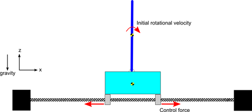
Figure 1: Inverted pendulum model setup
The pre-designed controller generates a control force that keeps the pendulum upright. The controller uses the pendulum’s orientation and angular velocity along with the cart’s displacement and velocity as inputs to calculate the direction and magnitude of the force needed to keep the pendulum upright. A block diagram of the control system is shown in Figure 2.
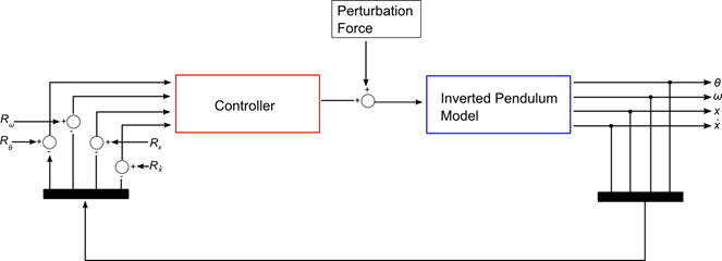
Figure 2: Block diagram representation of the controller
In the image above:
| • |  is the angular displacement of the pendulum from its model configuration is the angular displacement of the pendulum from its model configuration |
| • |  is the angular velocity of the pendulum about its center of gravity as measured in the ground frame of reference is the angular velocity of the pendulum about its center of gravity as measured in the ground frame of reference |
| • |  is the translational displacement of the cart measured from its model configuration in the ground frame of reference is the translational displacement of the cart measured from its model configuration in the ground frame of reference |
| • |  is the translational velocity of the cart measured in the ground frame of reference is the translational velocity of the cart measured in the ground frame of reference |
| • |  is a reference signal for the pendulum’s angular displacement is a reference signal for the pendulum’s angular displacement |
| • |  is a reference signal for the pendulum’s angular velocity is a reference signal for the pendulum’s angular velocity |
| • |  is a reference signal for the cart’s translational displacement is a reference signal for the cart’s translational displacement |
| • |  is a reference signal for the cart’s translational velocity is a reference signal for the cart’s translational velocity |
A disturbance is added to the computed control force to assess the system response. The controller force acts on the cart body to control the displacement and velocity profiles of the cart mass.
In this exercise, you will do the following:
| • | Solve the baseline model in MotionSolve only (i.e., without co-simulation) by using the inverted pendulum model with a continuous controller modeled by a Force_Vector_OneBody element. You can use these results to compare to an equivalent co-simulation in the next steps. |
| • | Review a modified MotionSolve inverted pendulum model that mainly adds the Control_PlantInput and Control_PlantOutput entities that allow this model to act as a plant for Simulink co-simulation. |
| • | Review the controller in Simulink. |
| • | Perform a co-simulation and compare the results between the standalone MotionSolve model and the co-simulation model. |
Before you begin, copy all the files in the <installation_directory>\tutorials\mv_hv_hg\mbd_modeling\motionsolve\cosimulation folder to your working directory (referenced as <Working Directory> in the tutorial). Here, <altair> is the full path to the HyperWorks installation.
Step 1: Run the baseline MotionSolve model.
In this step, use a single body vector force (Force_Vector_OneBody) to model the control force in MotionSolve. The force on the cart is calculated as:
 , where
 is the disturbance force,
 is the control force,
 are gains applied to each of the error signals
 is the error (difference between reference and actual values) on the input signals.
The angular displacement and velocity of the pendulum are obtained by using the AY() and WY() expressions respectively. The translational displacement and velocity of the cart are obtained similarly, by using the DX() and VX() expressions.
| 1. | From the Start menu, select All Programs > Altair HyperWorks 14.0 > MotionView. Open the model InvertedPendulum_NoCosimulation.mdl from your <Working Directory>. |
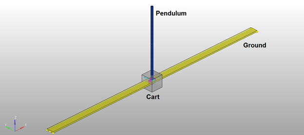
Figure 3: The MotionSolve model of the inverted pendulum
The MotionSolve model consists of the following components:
Component name
|
Component Type
|
Description
|
Slider cart
|
Rigid body
|
Cart body
|
Pendulum
|
Rigid body
|
Pendulum body
|
Slider Trans Joint
|
Translational Joint
|
Translational joint between the cart body and the ground
|
Pendulum Rev Joint
|
Revolute Joint
|
Revolute joint between the pendulum body and the cart body
|
Control Force
|
Vector Force
|
The control force applied to the cart body
|
Output control force
|
Output request
|
Use this request to plot the control force
|
Output slider displacement
|
Output request
|
Use this request to plot the cart’s displacement
|
Output slider velocity
|
Output request
|
Use this request to plot the cart’s velocity
|
Output pendulum displacement
|
Output request
|
Use this request to plot the pendulum’s displacement
|
Output pendulum velocity
|
Output request
|
Use this request to plot the pendulum’s velocity
|
Pendulum Rotation Angle
|
Solver Variable
|
This variable stores the rotational displacement of the pendulum via the expression AY()
|
Pendulum Angular Velocity
|
Solver Variable
|
This variable stores the rotational velocity of the pendulum via the expression VY()
|
Slider Displacement
|
Solver Variable
|
This variable stores the translational displacement of the cart via the expression DX()
|
Slider Velocity
|
Solver Variable
|
This variable stores the translational velocity of the cart via the expression VX()
|
| 2. | In the Run Panel, specify the name InvertedPendulum_NoCosimulation.xml for the MotionSolve model name and click Run. |
The results that we get from Step 2 will be used as the baseline to compare the results that we get from co-simulation.
Step 2: Use modified MotionSolve Model to define the plant in the control scheme.
A MotionSolve model needs a mechanism to specify the input and output connections to the Simulink model. The MotionSolve model (XML) used above is modified to include the Control_PlantInput and Control_PlantOutput model elements and provide these connections. In this tutorial, this has already been done for you, and you can see this by opening the model InvertedPendulum_Cosimulation.mdl from your <Working_Directory>.
This model contains two additional modeling components:
Component name
|
Component Type
|
Description
|
Plant Input Simulink
|
Plant input
|
This Control_PlantInput element is used to define the inputs to the MotionSolve model
|
Plant Output Simulink
|
Plant output
|
This Control_PlantOutput element is used to define the outputs from the MotionSolve model
|
| • | The Control_PlantInput element defines the inputs to a mechanical system or plant. For this model, only one input is defined in the “Plant Input Simulink” solver array. This is set to the ID of the solver variable that holds the control force from Simulink. |
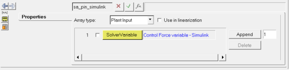
Figure 4: The definition of the input channel to MotionSolve
| • | The Control_PlantOutput element defines the outputs from a mechanical system or plant. For this model, four outputs are defined in the “Plant Output Simulink” solver array. These are the pendulum rotation angle, the pendulum angular velocity, slider displacement and slider velocity. |
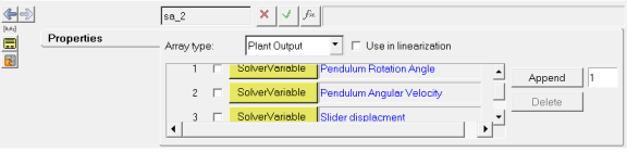
Figure 5: The definition of the output channels from MotionSolve
The inputs specified using the Control_PlantInput and Control_PlantOutput elements can be accessed using the PINVAL() and POUVAL() functions, respectively. Since the Control_PlantInput and Control_PlantOutput list the ids of solver variables, these input and output variables may also be accessed using the VARVAL() function. For more details, please refer to the MotionSolve User's Guide on-line help.
In this model, we have the following connections:
| • | Plant Input: A single control force that will be applied to the cart. |
| • | Plant Output: The pendulum’s angular displacement and angular velocity; the cart’s translational displacement and velocity. |
Step 3: Setting up environment variables to run MotionSolve from MATLAB\Simulink.
A few environment variables are needed for successfully running a co-simulation using MATLAB. These can be set using one of the following methods:
| • | In the shell/command window that calls MATLAB (with the set command on Windows, or the setenv command on Linux) |
| • | Within MATLAB, via the setenv() command |
An example of the usage of these commands is listed below:
Environment variable
|
Value
|
Windows shell
|
Linux shell
|
MATLAB shell
|
PATH
|
\mypath
|
set PATH=\mypath
|
setenv PATH \mypath
|
setenv(‘PATH’,’\mypath’)
|
Set the following environment variables
Environment variable
|
Path
|
|
|
Windows
|
Linux
|
NUSOL_DLL_DIR
|
<altair>\hwsolvers\motionsolve\bin\win64
|
<altair>\hwsolvers\motionsolve\bin\linux64
|
RADFLEX_PATH
|
<altair>\hwsolvers\common\bin\win64
|
<altair>\hwsolvers\common\bin\linux64
|
PATH
|
<altair>\hwsolvers\common\bin\win64;%PATH%
|
<altair>\hwsolvers\common\bin\linux64;$PATH
|
LD_LIBRARY_PATH
|
-
|
<altair>\hwsolvers\motionsolve\bin\linux64: <altair>\hwsolvers\common\bin\linux64:$LD_LIBRARY_PATH
|
where <altair> is the full path to the HyperWorks installation. For example, on Windows, this would typically be C:\Program Files\Altair\14.0.
Note that other optional environment variables may be set for your model. See MotionSolve Environment Variables for more information on these environment variables.
Step 4: Perform the co-simulation.
The core feature in Simulink that creates the co-simulation is an S-Function (System Function) block in Simulink. This block requires an S-Function library (a dynamically loaded library) to define its behavior. MotionSolve provides this library, but the S-Function needs to be able to find it. To help MATLAB/Simulink find the S-Function, you need to add the location of the S-Function to the list of paths that MATLAB/Simulink uses in order to search for libraries.
The S-Function libraries for co-simulation with MotionSolve are called either:
mscosim – for Shared Memory (SMP) communication
mscosimipc – for Inter Process Communication (IPC) using TCP/IP sockets for communication. Please see the tutorial MV-7003 for details on how to use IPC for co-simulation. The rest of this tutorial is described for the Shared Memory (SMP) communication process.
Changing the name of this library in the S-Function block in Simulink changes the communication behavior of the co-simulation.
These files are installed under <altair>\hwsolvers\motionsolve\bin\<platform>.
The location of these files needs to be added to the search path of MATLAB for the S-Function to use mscosim.
This can be done in one of the following ways:
| a. | From the Matlab menu, select File > Set Path…This is shown in Figure 6 below. |
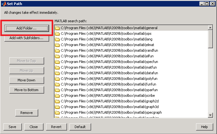
Figure 6: Add path through the MATLAB GUI
| b. | From the dialog box, add the directory where the mscosim libraries reside. |
(for example, <altair>\hwsolvers\motionsolve\bin\win64).
| c. | Select Save and Close. This procedure permanently adds this directory to the MATLAB/Simulink search path. |
At the MATLAB command line, type:
addpath(‘<altair>\hwsolvers\motionsolve\bin\<platform>’)
to add the directory where mscosim library resides into the MATLAB search path. It remains valid until you exit MATLAB. You can also create a .m script to make this process more easily repeatable.
For example, you can set the MATLAB Path and the necessary environment variables using MATLAB commands in a MATLAB (.m) script:
addpath('<altair>\hwsolvers\motionsolve\bin\win64')
setenv('NUSOL_DLL_DIR','<altair>\hwsolvers\motionsolve\bin\win64')
setenv('RADFLEX_PATH',['<altair>\hwsolvers\common\bin\win64')
setenv('PATH',['<altair >\hwsolvers\common\bin\win64;' getenv('PATH')])
For a Linux machine, additionally:
setenv(‘LD_LIBRARY_PATH’, '<altair>\hwsolvers\motionsolve\bin\linux64:<altair>\hwsolvers\common\bin\linux64\')
Step 5: View the controller modeled in Simulink
| 1. | In the MATLAB window, select File > Open. |
The Open file… dialog is displayed.
| 2. | Select the InvertedPendulum_ControlSystem.mdl file from your <Working Directory>. |
You will see the control system that will be used in the co-simulation.
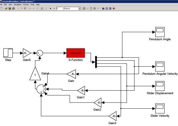
Figure 7: The control system in MATLAB
| 4. | The model contains an S-function block. Name the S-function ‘mscosim’. |
The S-function (system-function) is one of the blocks provided by Simulink and represents the MotionSolve model. It can be found in the Simulink User-Defined Functions block library. An S-Function allows you to model any general system of equations with inputs, outputs, states, and so on, and is somewhat analogous to a Control_StateEqn in MotionSolve. See the MATLAB/Simulink documentation for more details.
| 5. | Double-click the S-function with name mscosim. In the dialog box that is displayed, under the S Function Parameters, enter the following using single quotes: |
' InvertedPendulum_Cosimulation.xml', ' InvertedPendulum_Cosimulation.mrf', ''
The three parameters are the following:
| 1. | MotionSolve XML model name |
| 3. | MotionSolve user DLL name (optional); enter empty single quotes ('') if not used. |
Step 6: Perform the co-simulation.
| 1. | Click Simulation > Start to start the co-simulation. Simulink uses ODE45 to solve the Simulink model. From this, the co-simulation should begin and MotionSolve should create an output .mrf file for post-processing. Set the Scopes in the Simulink model to display the results. Also, check the .log file to make sure no errors or warnings were issued by MotionSolve. |
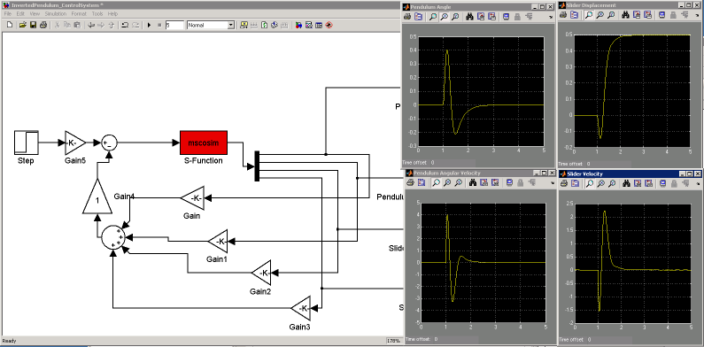
Figure 8: Running the co-simulation from Simulink
Step 7: Compare the MotionSolve-only results to the co-simulation results.
| 1. | From the Start menu, select All Programs > Altair HyperWorks 14.0 > HyperGraph. |
| 2. | Click the Build Plots icon,  . . |
| 3. | Click the file browser icon,  , and load the InvertedPendulum_NoCosimulation.mrf file. This was the baseline results created by running MotionSolve by itself. , and load the InvertedPendulum_NoCosimulation.mrf file. This was the baseline results created by running MotionSolve by itself. |
| 4. | In the Page Controls toolbar, create two vertical plot windows. |
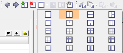
Figure 9: Create two plot windows
5. Select Marker Displacement for Y-Type, then REQ/70000004 Output slider displacement (on Slider cart) for Y Request, and DX for Y Component to plot the cart’s translational displacement:
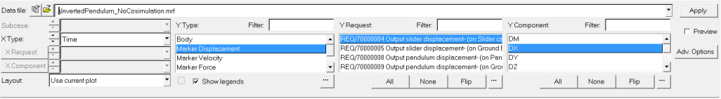
Figure 9: Plot the cart’s displacement
| 6. | Select the window on the left and click Apply. |
| 7. | Select Marker Force for Y-Type, then REQ/70000002 Output control force- (on Slider cart) for Y Request, and FX for Y Component to plot the X component of the control force: |
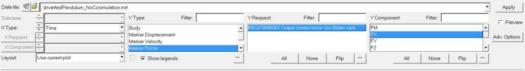
Figure 10: Plot the control force on the cart
| 8. | Click the file browser icon,  , and load the InvertedPendulum_Cosimulation.mrf file. This was the co-simulation results run with Simulink. , and load the InvertedPendulum_Cosimulation.mrf file. This was the co-simulation results run with Simulink. |
| 9. | Select Marker Displacement for Y-Type, then REQ/70000004 Output slider displacement (on Slider cart) for Y Request, and DX for Y Component to overlay the plot in the left window. |
| 10. | Select Marker Force for Y-Type, then REQ/70000002 Output control force- (on Slider cart) for Y Request, and FX for Y Component to overlay the plot in the right window. |
You will notice that both the signals match as shown below.
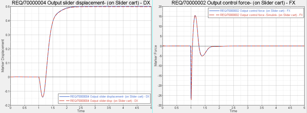
Figure 11: Comparison of the cart displacement and cart control force between the two models
The blue curves represent results from the MotionSolve-only model and the red curves represent results from the co-simulation.


