In this tutorial, you will learn the following:
| • | A brief introduction to Non-Linear Finite Element formulation used in MotionSolve. |
| • | Modeling NLFE bodies in MotionView. |
Introduction
Starting in version 14.0, MotionSolve introduced a new form of flexible body referred as Non Linear Finite Elements (NLFE). Unlike the conventional flexible body, where the body is represented in a modal form, NLFE is modeled in a direct Finite Element form.
NLFE Formulation
MotionSolve uses Absolute Nodal Coordinate Formulation (ANCF) to model large displacement and large deformation (NLFE) bodies. The absolute nodal coordinate formulation[1] is developed based on finite element formulation and is designed for large deformation multibody analysis. In the absolute nodal coordinate formulation, slopes and displacements are used as the nodal coordinates instead of infinitesimal or finite rotations.
ANCF uses the shape function matrix, together with the nodal coordinates to describe arbitrary rigid body motion. For these reasons, the absolute nodal coordinate formulation leads to a constant mass matrix in two- and three-dimensional cases. The constant mass matrix simplifies the nonlinear equations of motion and, consequently, accelerates the time integration of the nonlinear equations of motion.
Below is a standard beam model[2] described in 2D plane using ANCF.
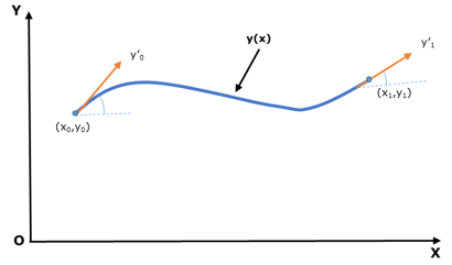
Euler–Bernoulli beam element
Displacement field, y(x) = s1(x)y0+ s2(x)y’0 +s3(x)y1+ s4(x)y’1
Where,
s1 to s4 are shape functions of beam.
x0, y0, x1, and y1 are nodal coordinates of 2 grids.
y’0 and y’1 are slope coordinates (gradients) at 2 grids.
The absolute nodal coordinate formulation has been applied to a wide variety of challenging nonlinear dynamics problems that include belt drives, rotor blades, elastic cables, leaf springs, and tires.
Non-linear finite element capabilities of MotionSolve
| • | All type of linear and non-linear elasticity is supported i.e. Isotropic, Orthotropic, Anisotropic and Hyper elasticity. |
| • | Geometric stiffening induced due to elastic forces. |
Modeling non-linear behavior above the elasticity limit (like plastic deformation, strain hardening, fracture etc.) is not supported. In the current version, MotionView supports modeling of 1D line elements only (Beam and Cable elements). Beam elements can have 18 types of cross-sections and the dimensions of the cross-section can be changed linearly in the axial direction. Beam elements can resist axial, shear, torsion and bending loads. The Cable element maintains a constant cross-section, thus it can resist only axial and bending loads.
This tutorial has two exercises:
| 1. | Cantilever beam bending. |
| 2. | Uniaxial tension of rubber. |
Exercise 1
In this exercise, you will model a 1m long cantilever beam with a cross-section dimension of 110mmx14mm to perform a bending test and compare it with an analytical solution.
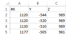
Copy the centerline.csv file, located in the mbd_modeling\nlfe\intro folder, to your <working directory>.
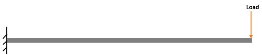
Cantilever beam under end load condition
Step 1: Modeling a Beam with Linear Elastic Material.
| 1. | Start a new MotionView session. |
| 2. | Right-click on the Body icon in the Model-Reference toolbar. |
The Add Body or BodyPair dialog is displayed.
| 3. | Specify the label as Cantilever Beam. |
| 4. | Specify the variable name as nlfeb_cantilever. |
| 5. | Select NLFE Body from the drop-down menu. |
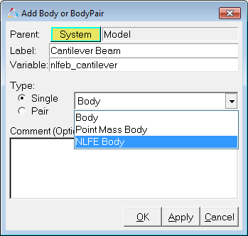
| 6. | Click OK to close the dialog. |
The NLFE Body is displayed with the Properties tab active.
The following table lists the various tabs available in the NLFE Body panel:
Tab name
|
Sets NLFEBody
|
Properties
|
Type (Beam/Cable), Cross-section, and material properties
|
Connectivity
|
Center line data or body profile
|
Orientation
|
Start and End orientations
|
Mass Properties
|
Displayed for information only
|
Initial conditions
|
Initial velocities
|
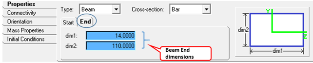
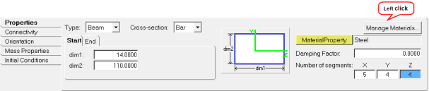
| 7. | From the Properties tab, define the properties as listed below: |
The panel also displays the image of the cross-section indicating what the different dimensions (dim1 and dim2) refer to.
| Note | The Properties tab has two sub-tabs called Start and End. These sub-tabs are used to set the dimensions at two different ends of the beam. By default, the End dimensions are parametrically equated to the Start dimensions. If a different set of dimensions are provided at the start and end, the cross section varies linearly along the length of the beam. |
| 8. | Click on the End sub-tab and review dim1 and dim2. |
| 9. | Click on the Manage Materials button located in the upper right corner of the Properties tab. |
The Material Properties dialog is displayed.
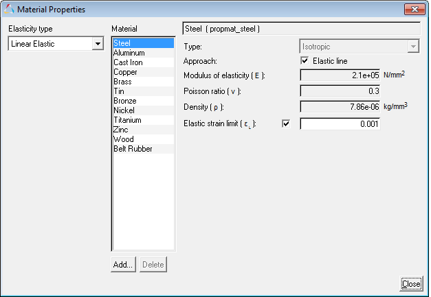
Note The Material Properties dialog can also be accessed from the Model menu.
MotionView provides a list of commonly used Linear Elastic, as well as Hyper Elastic material by default.
| 10. | Select Steel from the Material list. |
| 11. | Review the property values and notice that the Elastic line check box for Approach is selected. |
| 12. | Click Close to close the dialog. |
The default standard materials provided are defined with the Elastic Line option checked on. Materials without the Elastic Line are solved using the continuous mechanics approach, where in the cross-section deformation is taken into consideration. The Elastic Line approach ignores cross-section deformation effects, which gives results closer to an analytical solution.
| 13. | From the Connectivity tab, define the beam centerline by importing point data from a CSV file. Click on the Import Points button located in upper right corner. |
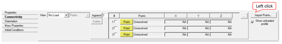
The Import Points From Coordinates In File dialog appears.
| 14. | Browse and select the centerline.csv file from your working directory. |
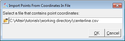
| 15. | Click OK to import the points. |
The .csv file must be in the following format: the first column must hold the X-coordinates, the second column the Y-coordinates, and the third column the Z-coordinates. There can also be a header row that begins with a # indicating a commented line.
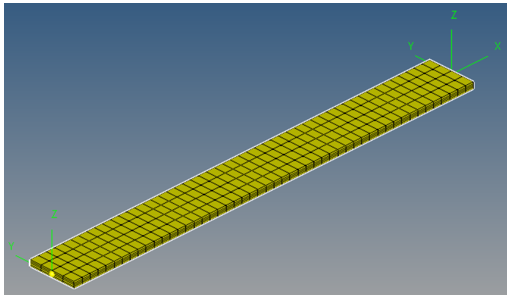
| 16. | Fit the model (by hitting 'F' on the the keyboard) to view the NLFE Body that was created. |
| 17. | Click on the Orientation tab to review the Start and End orientations. |
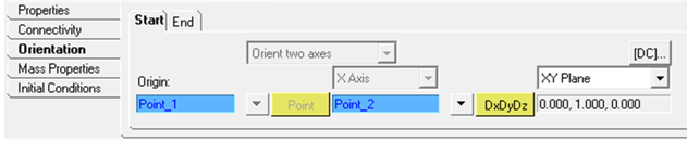
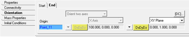
| Note | The Orientation tab is used to set the cross section orientation (YZ plane of the beam). Use the XY Plane or XZ Plane option to position the Y or the Z-axis (the remaining axis will be positioned so that it is orthonormal to the remaining two axes). |
Use the default orientation for this exercise.
Intermediate Beam elements orientation is linearly varied from Start orientation to End orientation. The Orientation option is useful in defining twist along the beam length.
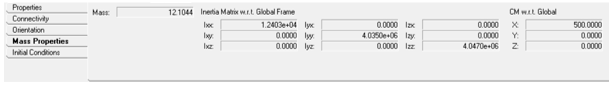
| 18. | Click on Mass Properties tab to review the calculated values. |
| 19. | Click on Initial Conditions tab to review the NLFEBody initial velocities. |
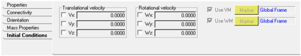
Leave initial velocities equal to zero.
Step 2: Adding a constraint and force.
| 1. | Create a Fixed joint at the beam origin point (Point_1) as specified in the table below: |
S.No
|
Label
|
Variable name
|
Type
|
Body 1
|
Body 2
|
Origin(s)
|
Orientation Method
|
Reference 1
|
Reference 2
|
1
|
Fix Joint
|
j_fix
|
Fixed Joint
|
Cantilever Beam
|
Ground Body
|
Point_1
|
|
|
|
| Note | Each grid on an NLFE body has 12 DOFs: 3 translational, 3 rotational, and 6 related to the length and angle between the gradient vectors. Using a fixed joint constrains the positions of the grid and the rigid body rotations. However, the gradients at the grid are free. This means that the cross-section at the fixed joint can twist about the grid and also deform based on Poisson’s ratio. To arrest these DOFs, an NLFE element called “CONN0” can be used. |
There is no graphical user interface support for creating this constraint. By default, MotionView creates a CONN0 element at all of those grids of the NLFE body through which it is attached to a constraint/force entity.
| 2. | Create a load at the cantilever beam end point (Point_11) as specified in the table below: |
S.No
|
Label
|
Variable name
|
Force
|
Properties
|
Action force on
|
Apply force at
|
Ref. Marker
|
1
|
Load
|
frc_load
|
Action only
|
Scalar Force along Z axis of Ref Frame
|
Cantilever Beam
|
Point_11
|
Global Frame
|
| 3. | From the Trans Properties tab, specify the expression for force as ` -1000*time`. |
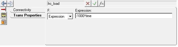
| Note | Negative value is specified to apply load along negative Z-axis direction. |
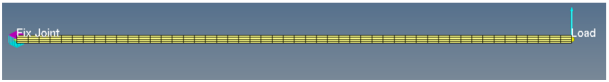
Cantilever beam with end load
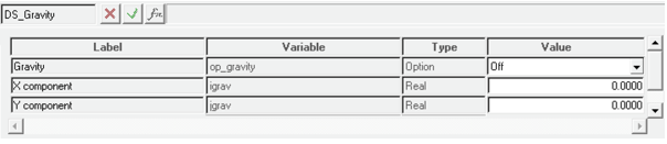
| 4. | Turn off gravity to eliminate deflection due to beam self-weight. |
Step 3: Creating outputs to measure cantilever beam end deflection.
Cantilever beam end deflection from linear-elasticity theory.
Deflection for load applied at end = 
Where,
 = Load (N)
 = Beam length = 1000mm
 = Youngs Modulus = 2.1e+05 N/mm2
 = Second Moment of Area =
  = 114 *
  = 25153.33mm4
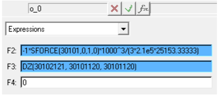
| 1. | Add an Output  of the Type Expressions with the following: of the Type Expressions with the following: |
| - | For Label, enter Deflection - Analytical (F2), NLFE(F3). |
| - | For F2, enter `-1*SFORCE({frc_load.idstring},0,1,0)*1000^3/(3*2.1e5*25153.33333)`. |
| - | For F3, enter `{frc_load.DZ}`. |
| 2. | Click on Check Model  to verify the model. to verify the model. |
| 3. | Add an output request Load to measure the magnitude of the applied Load. |
| 4. | Save  your model as nlfe_cantilever.mdl. your model as nlfe_cantilever.mdl. |
Step 4: Solving the model and post-processing.
The model is now complete and can be solved in MotionSolve.
| 1. | Invoke the Run panel by clicking on the Run Solver button  on the toolbar. on the toolbar. |
| 2. | Specify MotionSolve file name as Cantilever_beam.xml. |
| 3. | Select the Simulation type as Quasi-static, the end time as 1 sec, and the Print interval as 0.01. |
| 4. | Click on the Run button. |
| 5. | After the simulation is completed, click on the Animate button to view the animation in HyperView. |
| 6. | Click the Start/Pause Animation icon,  , on the Animation toolbar to start the animation. , on the Animation toolbar to start the animation. |
| 7. | Click the Plot button in the MotionView Run panel to load the .abf file in HyperGraph. |
| 8. | Plot Deflection vs Load calculated from linear elasticity theory and NLFE by selecting the data below in HyperGraph. |
Select following for X-axis data:
X Type
|
Marker Force
|
X Request
|
REQ/70000001 Load- (on Cantilever Beam)
|
X Component
|
FZ
|
Select the following Y-axis data:
Y Type
|
Expression
|
Y Request
|
REQ/70000000 Deflection – Analytical (F2), NLFE (F3)
|
Y Component
|
F2 & F3
|
| 9. | Click on the Define Curves toolbar icon  . . |
| 10. | Rename the two curves as Analytical and NLFE as shown below: |
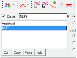
Define Curves panel
It can be observed from the plot that the NLFE and Analytical curves almost overlap.
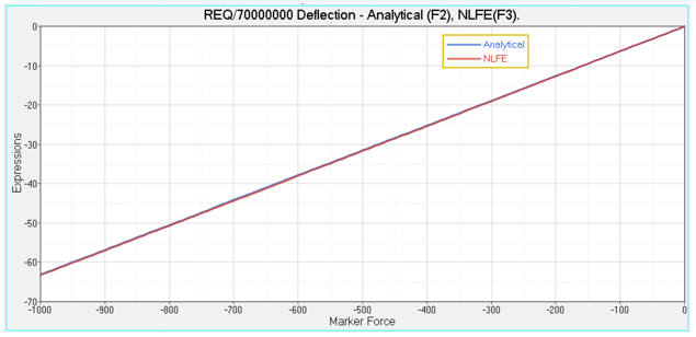
Deflection versus load plot
| 11. | Activate the Hyperview animation window. |
| 12. | Click on the Contour button  on the toolbar to activate the Contour panel. on the toolbar to activate the Contour panel. |
| 13. | Under Result type, select NLFE Stress (t) and XX. |
| 14. | Click Apply to view bending stress contours. |
Similarly, you can view Displacement, Strain, etc. for an NLFE body in HyperView. All FE contours and types are available in HyperView for an NLFE body.
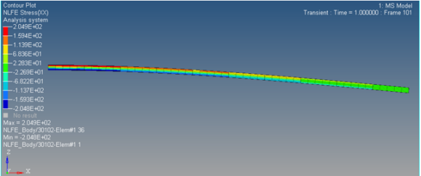
Bending stress contour of NLFE beam
| 15. | Save  this session as nlfe_cantilever.mvw. this session as nlfe_cantilever.mvw. |
Exercise 2: Tensile test of Elastomer
Hyper-elastic materials are large strain materials when compared to metals. In case of hyper-elastic materials the non-linear relation between stress and strain is derived from a strain energy density function. Currently MotionSolve supports three hyper-elastic material models: Neo-Hookean, Mooney–Rivlin, and Yeoh.
In this exercise, a uni-axial tensile test on a rubber strip (2mmx25mmx50mm) will be performed. Hyper-elastic material constants have been sourced from reference[3].
Clear the existing session through File>New>Session  .
.
Step 1: Adding a new material property.
| 1. | From the Main menu, select Model>Materials. |
| 2. | In Material Properties dialog: |
| - | For Elasticity type, select Hyper Elastic. |
| - | Click on the Add button. |
Adding new HyperElastic material
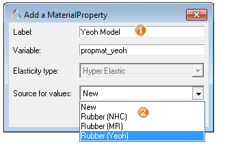
| 3. | From Add a MaterialProperty dialog: |
| - | Specify the Label as Yeoh Model and Variable name as propmat_yeoh. |
| - | For Source for values, select Rubber (Yeoh). |
| - | Click OK to add the material property. |
Selecting source values for new material
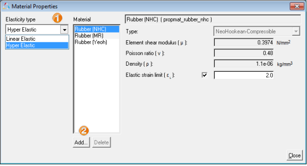
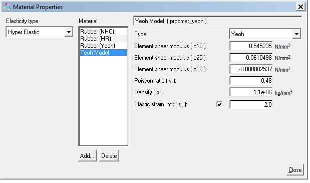
| 4. | Specify the following values for this material: |
| - | Element shear modulus (c10): 0.545235 |
| - | Element shear modulus (c20): 0.0610498 |
| - | Element shear modulus (c30): −0.000802537 |
| - | Poisson ratio ( ): 0.48 ): 0.48 |
| - | Density ( ): 1.1e-6 ): 1.1e-6 |
| - | Elastic strain limit (εL): 2.0 |
Specifying material constant values
Step 2: Modeling the rubber strip.
| 1. | Create two points for the rubber strip length profile with the details show in the table below. |
S.No
|
Label
|
Variable name
|
x
|
y
|
z
|
1
|
Rubber End 1
|
p_rub_end1
|
0.0
|
0.0
|
0.0
|
2
|
Rubber End 2
|
p_rub_end2
|
50.0
|
0.0
|
0.0
|
| 2. | Create 9 intermediate points between the above points using the Create Points Along a Vector  macro. macro. |
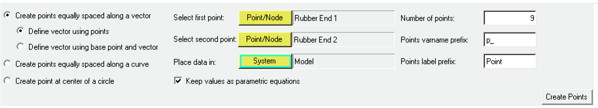
Creating intermediate points using “Create Points along a Vector” macro.
| 3. | Right-click on the Body icon  in the Model-Reference toolbar. Add a new NLFE body with the Label as Rubber Strip and the Variable name as nlfeb_rubber_yeoh. in the Model-Reference toolbar. Add a new NLFE body with the Label as Rubber Strip and the Variable name as nlfeb_rubber_yeoh. |
In the Properties tab, specify the properties below:
| - | Select the Yeoh Model created in previous step as the MaterialProperty. |
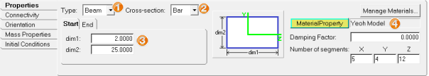
Specifying beam properties
| - | Go to Connectivity tab; Append 8 more points to the displayed table. |
| - | Activate the first Point collector and select the point Rubber End 1. |
| - | Select the next available intermediate points one by one into other collectors, with the last point being Rubber End 2. |
Rubber strip model
Step 3: Adding constraints.
| 1. | Create Fix joint at one end and Translation joint at other as specified in below table: |
S.No
|
Label
|
Variable name
|
Type
|
Body 1
|
Body 2
|
Origin(s)
|
Orientation Method
|
Reference 1
|
Reference 2
|
1
|
Fix Joint
|
j_fix
|
Fixed Joint
|
Rubber Strip
|
Ground Body
|
Rubber End 1
|
|
|
|
2
|
Translation Joint
|
j_trans
|
Translational joint
|
Rubber Strip
|
Ground Body
|
Rubber End 2
|
Alignment axis (Vector)
|
Global X
|
|
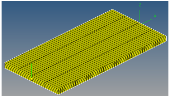
| 2. | Create motion on the Translation joint to apply axial pull. |
S.No
|
Label
|
Variable name
|
Define Motion
|
Joint
|
Property
|
1
|
Axial Motion
|
mot_axial
|
On Joint
|
Translation Joint
|
Displacement
|
| 3. | In Properties tab, specify the following properties: |
Motion expression
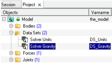
| 4. | Go to the Solver Gravity  dataset and change the Gravity option to Off. dataset and change the Gravity option to Off. |
| 5. | Click the Save Model icon on the Standard toolbar and save your model as rubber_strip.mdl in your <working directory>. |
Step 4: Adding outputs.
Create outputs to measure engineering strain and engineering stress values.
Engineering Strain = 
Engineering Stress = 
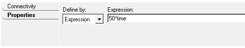
| 1. | Add an Output of the Type Expressions with the Label as Eng strain(F2), Eng Stress (F3) and the expressions as shown below: |
| - | F2: `(DM({j_trans.i.idstring},{j_fix.i.idstring})-50)/50` |
| - | F3: `MOTION({mot_axial.idstring},{0},{2},{0})/50` |
Output requests
| Note | In the above expression F2, the solver function DM() measures the distance magnitude between two markers; the I marker of the Translation Joint and the I marker of the Fix Joint. Expression F3 uses the solver function MOTION() which measures the reaction force due to the imposed motion Axial Motion. |
Step 5: Solving the model and post-processing.
| 1. | To solve the model, go to Run panel . |
| 2. | Specify the MotionSolve file name as rubber_yeoh.xml. |
| 3. | Select the Simulation type as Transient; the End time: 4, and the Print interval: 0.01. |
| 5. | As the solver is executing, a warning message similar to the one shown below may be displayed: |
WARNING: Maximum vonMises strain exceeded maximum strain (YS) specified for NLFE element BEAM12 (id=20000000) on Body_Flexible (id=30102) at time=1.183E+00
Maximum strain Computed : 2.015E+00
Maximum strain Specified: 2.000E+00
Future warning for yield strain violation suppressed.
This message states that the maximum vonMises strain in your NLFE component exceeded what was specified (2.0) at time 1.18s. This message lets you know if your component is deforming more than what you would expect it to, which allows you to inspect your results and make corrections in modeling your system if required.
| 6. | After the simulation is completed, click on Animate to view the animation in HyperView. |
| 7. | Click the Start/Pause Animation button to play the animation. |
| 8. | Go to the Contour panel and select NLFE Stress (t), XX, and click Apply. |
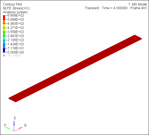
Stress contour
| 9. | Return to MotionView Run panel and click on Plot button to load the .abf file in HyperGraph. |
| 10. | Plot Engineering Stress vs Engineering Strain by selecting the data below in HyperGraph. |
| - | Select following for X-axis data: |
X Type
|
Expression
|
X Request
|
REQ/70000000 Eng strain(F2), Eng Stress(F3)
|
X Component
|
F2
|
| - | Select the following Y-axis data: |
Y Type
|
Expression
|
Y Request
|
REQ/70000000 Eng strain(F2), Eng Stress(F3)
|
Y Component
|
F3
|
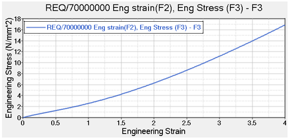
Stress versus strain curve
| Note | The animation shows the true stress due to cross-section deformation. |
| 11. | Save the model. |
| 12. | Save this session as hyperelastic.mvw. |
References:
| 1) | JUSSI T, SOPANEN and AKI M. MIKKOLA: Description of Elastic Forces in Absolute Nodal Coordinate Formulation. Journal of Nonlinear Dynamics 34: 53–74, 2003. |
| 2) | Oleg Dmitrochenko:Finite elements using absolute nodal coordinates for large-deformation flexible multibody dynamics. Proceedings of the Third International Conference on Advanced Computational Methods in Engineering (ACOMEN 2005). |
| 3) | Sung Pil Jung, TaeWon Park, Won Sun Chung: Dynamic analysis of rubber-like material using absolute nodal coordinate formulation based on the non-linear constitutive law. Journal of Nonlinear Dyn (2011) 63: 149–157. |


