MV-1027: Modeling Point-to-Deformable-Curve (PTdCV) Higher-Pair Constraint

In this tutorial, you will learn how to:

•	Model a PTdCV (point-to-deformable-curve) joint

A PTdCV (point-to-deformable-curve) joint is a higher pair constraint. This constraint restricts a specified point on a body to move along a specified deformable curve on another body. The curve may be open or closed, planar or in 3-d space. The point may belong to a rigid, flexible or a point mass. For this, we define a deformable curve on a beam supported at its ends by revolute joints. A mass is constrained to move along the curve with a PTdCV constraint.

Exercise

Copy the file KG_N_MM_S_50elems2.h3d, located in the mbd_modeling\interactive folder, to your <working directory>.

Step 1: Creating points.

Let’s start with creating points that will help us locate the bodies and joints as required. We will define points for center of mass of the bodies and joint locations.

1.	Start a new MotionView Session. We will work with the default units (kg, mm, s, N).

2.	From the Project Browser right-click on Model and select Add Reference Entity > Point (or right-click the Points icon on the Model-Reference toolbar).

The Add Point or PointPair dialog is displayed.

3.	For Label, enter PointbeamInterface1.

4.	Accept the default variable name and click OK.

5.	Click on the Properties tab and specify the coordinates as X = 152.4, Y, = 0.0, and Z = 0.0.

6.	Follow the same procedure for the other points specified in the table below:

Point	X	Y	Z
PointbeamInterface2	460.80	0.0	0.0
Point0	183.24	0.0	0.0
Point1	214.08	0.0	0.0
Point2	244.92	0.0	0.0
Point3	275.76	0.0	0.0
Point4	306.60	0.0	0.0
Point5	337.44	0.0	0.0
Point6	368.28	0.0	0.0
Point7	399.12	0.0	0.0
Point8	429.96	0.0	0.0

Step 2: Creating Bodies.

We will have two bodies apart from the ground body in our model visualization: the beam and the ball. Pre-specified inertia properties will be used to define the ball.

1.	From the Project Browser right-click on Model and select Add Reference Entity > Body (or right-click the Body icon on the Model-Reference toolbar).

The Add Body or BodyPair dialog is displayed.

2.	For Label, enter Beam and click OK.

3.	Accept the default variable name and click OK.

For the remainder of this tutorial - accept the default names that are provided for the rest of the variables that you will be asked for.

4.	From the Properties tab, check the Deformable box.

5.	Click on the Graphic file browser icon , select KG_N_MM_S_50elems2.h3d from the <working directory> and click Open.

The same path will automatically appear next to the H3D file browser icon .

6.	Right-click on Bodies in the Project Browser and select Add Body.

The Add Body or BodyPair dialog is displayed.

7.	For Label, enter Ball and click OK.

8.	From the Properties tab, specify the following for the Ball:

Body	Mass	Ixx	Iyy	Izz	Ixy	Iyz	Izx
Ball	100	1e6	1e6	1e6	0.0	0.0	0.0

9.	For the Ball body, under the CM Coordinates tab, check the Use center of mass coordinate system box.

10.	Double click on Point.

The Select a Point dialog is displayed.

11.	Choose Point4 and click OK.

12.	Accept defaults for axes orientation properties.

13.	For the Ball body, from the Initial Conditions tab - check the Vx box under Translational velocity and enter a value of 100 into the text box.

This sets a value of 100 for the translational velocity of the ball in the X-direction. A somewhat high value of Vx is introduced to make the motion of the ball clearly visible in the animation.

14.	Accept all the other default values.

Step 3: Creating Markers.

Now, we will define some markers required for the beam. We will totally define eleven markers here at equal distances along the span of the beam.

1.	From the Project Browser right-click on Model and select Add Reference Entity > Marker (or right-click the Markers icon on the Model-Reference toolbar).

The Add Marker or MarkerPair dialog is displayed.

2.	For Label, enter Marker0 and click OK.

3.	Under the Properties tab, double-click on Body.

The Select a Body dialog is displayed.

4.	Choose Beam and click OK.

5.	Under the Properties tab, double-click on Point.

The Select a Point dialog is displayed.

6.	Choose PointbeamInterface1 and click OK.

Accept the defaults for axes orientation.

7.	Right-click on Markers in the Project Browser and select Add Marker to define a second marker. Continue adding markers until Marker10 is reached.

8.	For subsequent labels; enter Marker1, Marker2, etc. until Marker10 is reached.

9.	From the Properties tab, always select the Beam (after double-clicking on Body each time).

10.	From the Properties tab, select Point0 through Point8, and finally PointbeamInterface2 for Marker10 (by double-clicking on Point every time).

Always accept the defaults for axes orientation.

A table is provided below for reference:

Marker No.	Body	Point
0	Beam	PointbeamInterface1
1	Beam	Point0
2	Beam	Point1
3	Beam	Point2
4	Beam	Point3
5	Beam	Point4
6	Beam	Point5
7	Beam	Point6
8	Beam	Point7
9	Beam	Point8
10	Beam	PointbeamInterface2

Step 4: Creating Joints.

Here, we will define all the necessary joints except for the PTdCV joint, which will be defined as an advanced joint later. We require two joints for the model, both of them being fixed joints between the beam and ground body.

1.	From the Project Browser right-click on Model and select Add Constraint > Joint (or right-click the Joints icon on the Model-Constraint toolbar).

The Add Joint or JointPair dialog is displayed.

2.	For Label, enter Joint0.

3.	Select Fixed Joint as the type and click OK.

4.	From the Connectivity tab, double-click on Body 1.

The Select a Body dialog is displayed.

5.	Choose Beam and click OK.

6.	Under the Connectivity tab, double-click on Body 2.

The Select a Body dialog is displayed.

7.	Choose Ground Body and click OK.

8.	From the Connectivity tab, double-click on Point.

The Select a Point dialog is displayed.

9.	Choose PointbeamInterface1 and click OK.

10.	Right-click on Joints in the Project Browser and select Add Joint to define a second joint.

The Add Joint or JointPair dialog is displayed.

11.	For Label, enter Joint1.

12.	Select Fixed Joint as the type and click OK.

13.	From the Connectivity tab, double-click on Body 1.

The Select a Body dialog is displayed.

14.	Choose Beam and click OK.

15.	From the Connectivity tab, double-click on Body 2.

The Select a Body dialog is displayed.

16.	Choose Ground Body and click OK.

17.	From the Connectivity tab, double-click on Point.

The Select a Point dialog is displayed.

18.	Choose PointbeamInterface2 and click OK.

Step 5: Creating Deformable Curves.

Here we will now define the deformable curve on the surface of the beam. The ball is constrained to move along this curve.

1.	Click the Project Browser tab, right-click on Model and select Add Reference Entity > Deformable Curve (or right-click the Deformable Curves icon on the Model-Reference toolbar).

The Add DeformableCurve dialog is displayed.

2.	For Label, enter DeformableCurve0, and click OK.

3.	From the Properties tab, select Marker for Data type, and NATURAL for Left end type and Right end type.

4.	Check the box just to the left of the Marker collector (which situated to the far right of Data Type).

The intermediate Add button is changed to an Insert button.

5.	Enter 10 into the text box located just to the right of the Insert button, and then click on the Insert button.

Eleven Marker collectors are displayed.

6.	Click on the individual collectors.

The Select a Marker dialog is displayed.

7.	Select all the markers one by one, starting from Marker 0 to Marker 10.

Step 6: Creating Advanced Joints.

Now we will define the advanced PTdCV joint.

1.	From the Project Browser right-click on Model and select Add Constraint > Advanced Joint (or right-click the Advanced Joints icon on the Model-Constraint toolbar).

The Add AdvJoint dialog is displayed.

2.	For Label, enter AdvancedJoint 0.

3.	From the Connectivity tab select: PointToDeformableCurveJoint, Ball for Body, Point4 for Point, and DeformableCurve 0 for DeformableCurve.

Step 7:Creating Graphics.

Graphics for the ball will now be built here.

1.	Click the Project Browser tab, right-click on Model and select Add Reference Entity > Graphic (or right-click the Graphics icon on the Model-Reference toolbar).

The Add Graphics or GraphicPair dialog is displayed.

2.	For Label, enter Graphic0.

3.	For Type, choose Sphere from the drop-down menu and click OK.

4.	From the Connectivity tab, double-click on Body.

The Select a Body dialog is displayed.

5.	Choose Ball and click OK.

6.	Again from the Connectivity tab, double-click on Point.

The Select a Point dialog is displayed.

7.	Choose Point4 and click OK.

8.	From the Properties tab, enter 2.0 as the radius of the Ball.

9.	From the Visualization tab, select a color for the Ball.

Step 8: Return to the Bodies Panel.

1.	Click the Body icon on the Model-Reference toolbar.

2.	For the beam which has already been defined, click on the Nodes button.

The Nodes dialog is displayed.

3.	Uncheck the Only search interface nodes box and then click on Find All.

4.	Close the the Nodes dialog.

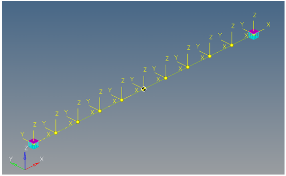
At the end of these steps your model should look like the one shown in the figure below:

mv-1027_pic1

One final comment before running the model:

This type of constraint does not ensure that the contact point will stay within the range of data specified for the curve. Additional forces at the end need to be defined by the user to satisfy this requirement. If the contact point goes out of range of the data specified for this curve, the solver encounters an error (unless additional forces are defined to satisfy this). In that case, one has to change the initial velocities for the ball, or increase the range of data specified for the curve, or run the simulation for a shorter interval of time.

Step 9: Running the Model.

We now have the model defined completely and it is ready to run.

1.	Click the Run icon on the Model-Main toolbar.

The Run panel is displayed.

2.	From the Main tab, specify values as shown below:

mv-1027_pic2

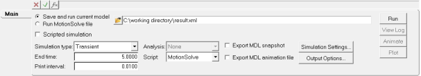
3.	Choose the Save and run current model radio button.

4.	Click on the browser icon and save the file as result.xml.

5.	Click Save.

6.	Click the Check Model button on the Model Check toolbar to check the model for errors.

7.	To run the model, click the Run button on the panel.

The solver will get invoked here.

Step 10: Viewing the Results.

1.	Once the solver has finished its job, the Animate button will be active. Click on Animate.

The icon can be used to start the animation, and the icon can be used to stop/pause the animation.

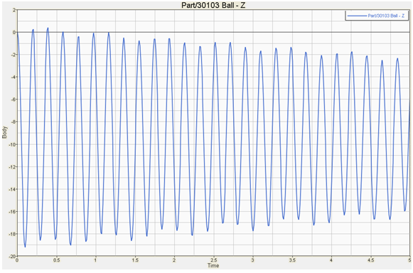
One would also like to inspect the displacement profile of the beam and the ball. For this, we will plot the Z position of the center of mass of the ball.

2.	Click on the Add Page icon and add a new page.

3.	Use the Select application drop-down menu to change the application from MotionView to HyperGraph 2D .

4.	Click the Build Plots icon on the Curves toolbar.

5.	Click on the browser icon and load the result.abf file.

6.	Make selections for the plot as shown below:

mv-1027_pic3

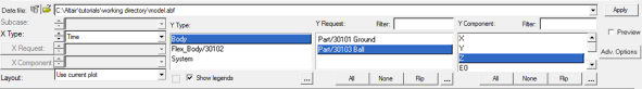
We are plotting the Z position of the center of mass of the ball.

7.	Click Apply.

The profile for the Z-displacement of the ball should look like the one shown below:

mv-1027_pic4