MV-7007: Adding Friction to Joints

In this tutorial, you will learn more about:

•	The MotionSolve joint friction model.

•	How to model Joint friction in MotionView/MotionSolve.

•	How to review the friction results.

Introduction

Friction is defined as a resistance force opposing motion. Friction appears at the physical interface between any two surfaces in contact. Friction force arises mainly due to adhesion, surface roughness and plowing at the contact surfaces.

1.	When contacting surfaces are smoother and brought to closer proximity; molecular adhesive forces forms resistance to motion.

2.	When contact surfaces are highly rough to cause abrasion on sliding; surface roughness resists motion.

3.	When one surface in contact is relatively soft, plowing effect causes most of resistance.

Friction forces generated depend on:

•	Surface contact geometry and topology

•	Properties of the bulk and surface materials

•	Displacement and relative velocity

•	Lubrication

Friction is highly non-linear and dependents on system states like stiction regime, transition regime and sliding (or) dynamic regime.

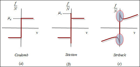
mv-7007_friction_function_characteristics_example

The three characteristics of a friction function

The friction force varies based on its states (as shown in the above figure). The (a) section shows Coulomb friction, (b) shows Stiction plus Coulomb friction, and F(c) shows how the friction force may decrease continuously from the static friction level due to lubrication also known as Stribeck effect.

Dynamics of friction

Friction-velocity relation or damping characteristics of friction will aid in dampening vibrations. There are other behaviors of friction such as pre-sliding and hydrodynamic effects of lubrications during dynamic simulations. Resistant forces from the above mentioned effects need consideration in design of drive systems and high-precision servo mechanisms. So, it’s important to model friction accurately to capture system dynamics.

Joint friction

Friction in joint depends on its geometry. MotionSolve uses an analytical model to represent friction for different joints based on geometry, preloads, torque and lubrication.

Characterizing joint friction using LuGre friction model

MotionSolve uses LuGre model for friction representation. LuGre model is a bristle model emerged for controls applications. LuGre model was presented by Canudas de Wit, Olsson, Åstro¨m, and Lischinsky. Stemming from a collaboration among researchers at the Lund Institute of Technology (Sweden) and in Grenoble France (Laboratoire d’Automatique de Grenoble), the LuGre model captures a variety of behaviors observed in experiments, from velocity and acceleration dependence of sliding friction, to hysteresis effects, to pre-slip displacement and lubrication.

mv-7007_diagram

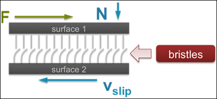
The Bristle model for friction

LuGre model can model friction considering geometry of joint, preload, moment arm, force and torque. Friction is supported for a subset of joints namely Revolute, Spherical, Translational Joint, Cylindrical, and Universal Joint. Please refer to our MotionSolve online help for a detailed explanation of friction for each constraint.

This tutorial uses an experimental model of a “block sliding on a table” to demonstrate friction forces under stick-slip condition and frequency dependency of friction forces.

Exercise

Copy the SlidingTable.mdl file, located in the mbd_modeling\motionsolve folder, to your <working directory>.

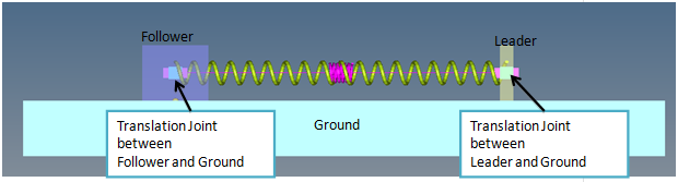
mv-7007_sliding_block_model_example

The leader and follower model constitutes two rigid bodies namely Leader and Follower respectively connected to the Ground body by translation joints and inter connected by a linear spring. In the following steps you will add friction and apply motions to study friction behavior of the translation joint.

Step 1: Adding Joint Friction.

1.	From the Project Browser, browse to the Joints folder and select Follower Translation Joint.

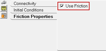
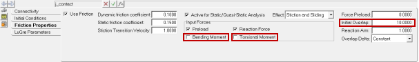
2.	From the Joints panel, go to the Friction Properties tab.

3.	From the Friction Properties tab, check the Use Friction option to activate friction on joint.

mv-7007_joints_panel_friction_props_tab

Note	MotionView populates the panel with default properties that are appropriate with units N, mm, second. You will need to scale properties such as Stiction Transition Velocity, Force Preload, and Geometric properties (Initial Overlap, Reaction Arm) according to the units.

4.	Uncheck the Bending Moment and Torsion Moment options to exclude joint reaction forces due to geometry misalignments. Modify the Initial Overlap value to 10mm and leave the remaining values at their default settings.

mv-7007_joints_panel_friction_props_tab_bending_torsion_moment

5.	Select the LuGre Parameters tab to modify the Bristle properties. Modify the Damping Coefficient value to 0.0316.

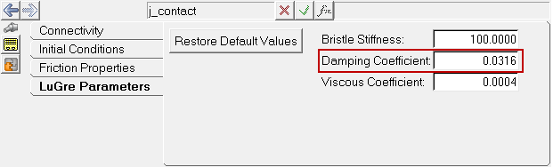
mv-7007_joints_panel_lugre_params_tab

Note	Default properties of bristle are appropriate with units N, mm, second.

6.	Leave all the LuGre parameters at their default values.

Step 2: Adding output requests for friction force.

In this step you will create an output to measure the friction forces on the Follower Translation Joint.

1.	Right click the Output icon from General MDL Entity Tool bar.

The Add Output dialog is displayed.

2.	Change the Label to Friction_Force.

3.	Change the Variable to o_friction.

mv-7007_add_output_dialog

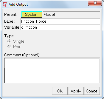
4.	Click OK to add output request.

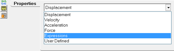
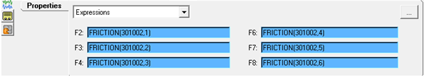
5.	From the Properties tab, select the output type as Expressions.

mv-7007_outputs_panel_properties_tab

6.	Click in the F2 expression field.

7.	Click on the button.

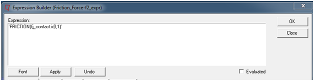
The Expression Builder dialog is displayed.

8.	Populate the Expression Builder with the FRICTION function expression as: `FRICTION({j_contact.id},1)`.

Follower Translation Joint ID	= {j_contact.id},
Fx component	= 1

mv-7007_expression_builder_friction_example

Click OK.

10.	Repeat the process for F3, F4, F6, F7, and F8 by changing the second parameter to 2, 3, 4, 5, and 6 accordingly.

The function FRICTION(ID, comp) computes the friction force component specified in the comp corresponding to the joint ID.

ID	The ID of the Joint.
comp	The force component. Currently, a range of 1-18 is supported.
	1 = Friction force FX along the x-axis of the J marker of the joint.
	2 = Friction force FY along the y-axis of the J marker of the joint.
	3 = Friction force FZ along the z-axis of the J marker of the joint.
	4 = Friction torque TX along the x-axis of the J marker of the joint.
	5 = Friction torque TY along the y-axis of the J marker of the joint.
	6 = Friction torque TZ along the z-axis of the J marker of the joint.

mv-7007_outputs_panel_properties_tab_expressions

Step 3: Adding output request for sliding velocity.

Friction forces are characterized with respect to the relative velocity between bodies under contact. So, you will create an output request to measure Follower body velocity.

1.	Right click the Outputs icon on the General MDL Entity toolbar.

The Add Output dialog is displayed.

2.	For Label, enter Follower_Velocity.

3.	For Variable, enter o_velocity.

4.	Click OK to add the output request.

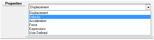
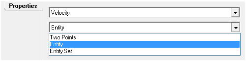
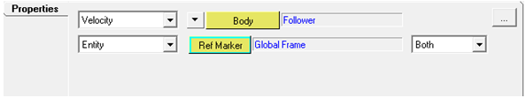
5.	From the Properties tab, select the output type as Velocity.

mv-7007_outputs_panel_properties_tab_velocity

6.	Select Entity from the drop-down menu below Velocity.

mv-7007_outputs_panel_properties_tab_velocity_entity

7.	Select entity type to be .

8.	Leave to be Global Frame.

mv-7007_outputs_panel_properties_tab_example2

Step 4: Add a constant velocity motion to the leader translation joint.

In this next step we will add constant velocity to the Leader Body. Follower body connected by a linear spring will observe a stick-slip motion due to the friction forces.

1.	Right click the Motion icon from the Constraint toolbar.

The Add Motion or MotionPair dialog is displayed.

2.	For Label, enter Stick Slip.

3.	For Variable, enter mot_leader.

4.	Click OK to add motion.

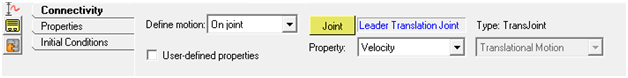
5.	From the Connectivity tab:

-	Select On Joint from the drop-down menu for Define motion.

-	Select Leader Translation Joint for .

-	Select Velocity from the drop-down for Property.

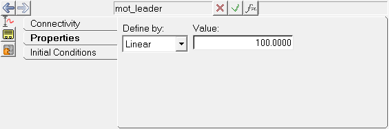
mv-7007_motion_panel_connectivity_tab

6.	From the Properties tab:

-	Select Linear from the drop-down menu for Define by.

-	Enter 100 for Value.

mv-7007_motion_panel_properties_tab

Step 5: Simulate the model.

1.	Click on the icon to check the model.

2.	Switch to the Run panel by clicking on the Run icon

3.	Under the Main tab, click on the icon to specify the name and location of the MotionSolve .xml file. Save the file with the name Stick_Slip.xml in your working directory.

mv-7007_run_panel_stick_slip

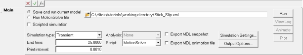
4.	Notice that after saving the file, the Run button to the right becomes active.

5.	Specify the End time as 25 sec and leave the other values at their default setttings.

6.	Click on the Run button to run the simulation.

Step 6: Viewing animation and plots.

Once the run is complete, the other buttons on the right side of the panel are activated.

1.	Click on the Animate button to view the animation.

This invokes HyperView and loads the Stick_Slip.h3d animation file.

2.	Next, click on the Plot button to view the plots.

This invokes HyperGraph and loads the Stick_Slip.abf results file.

3.	Click on the HyperGraph window to activate it.

4.	Plot Follower velocity versus Time.

-	Select X-axis Data Type as Time.

-	Select the following Y-axis data:

Y Type	Marker Velocity
Y Request	Follower_Velocity - (on Follower)
Y Component	VX

Note	Scale velocity value to m/sec from mm/sec.

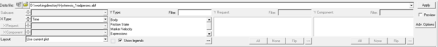
5.	Plot Friction force versus Time.

-	Select X-axis Data Type as Time.

-	Select the following Y-axis data:

Y Type	Expression
Y Request	Friction_Force
Y Component	F4

mv-7007_animation_plot_example

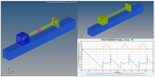
Animation and Plot windows

6.	To start the animation, click the Start/Pause Animation icon on the toolbar.

7.	The Stick_Slip motion is clearly observed from the animation and plots.

mv-7007_friction_force_graph

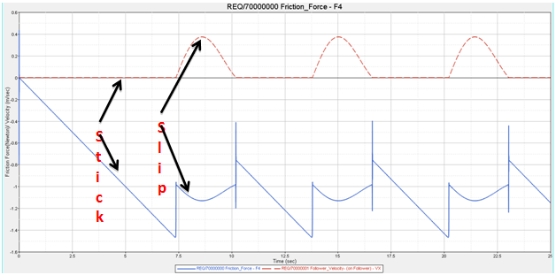
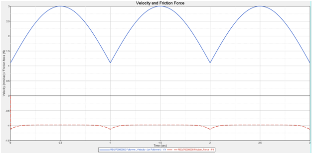
Velocity and Friction Force on Time Scale

The Leader body moving at a constant velocity elongates the spring increasing spring force linearly. The friction force counteracts the spring force, and there is a small displacement of Follower body when the applied force reaches the break-away force.

Break away force	= mu static x Normal Load
	= 0.15x1x9.81
	= 1.47 Newton.

Step 7: Adding time varying velocity to follower translation joint.

In this step you will add “Time varying velocity” to Follower translation joint. Velocity is varied between 1.1 mm/sec to 3mm/sec at different frequencies (1 rad/sec, 10 rad/sec & 25rad/sec) to observe Hysteresis in friction.

1.	Right-click the Motions icon on the Constraint toolbar.

The Add Motion or MotionPair dialog is displayed.

2.	For Label, enter Hysteresis.

3.	For Variable, enter mot_freq_varying.

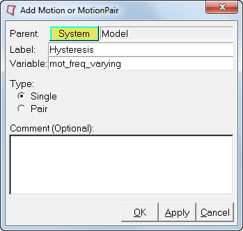
mv-7007_add_motion_or_motionpair_dialog

4.	Click OK to add motion.

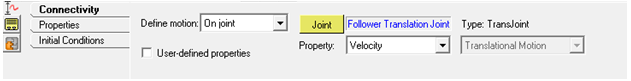
5.	From the Connectivity tab:

-	Select On Joint from the drop-down menu for Define motion.

-	Select Follower Translation Joint for .

-	Select Velocity from the drop-down for Property.

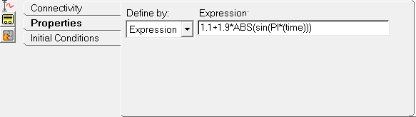
mv-7007_motion_panel_connectivity_tab_example2

6.	From the Properties tab:

-	Select Expression from the drop-down menu for Define by.

-	Click on the button.

The Expression Builder is displayed.

-	Populate the Expression Builder with the following expression: `1.1+1.9ABS(sin(PI(time)))`

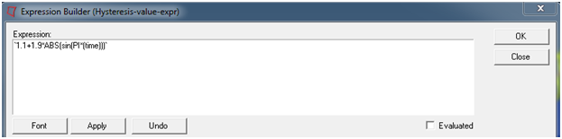
mv-7007_expression_builder_hysteresis_example

This expression varies velocity from 1.1 mm/sec to 3 mm/sec at a frequency of 1 rad/sec.

mv-7007_velocity_variation_graph

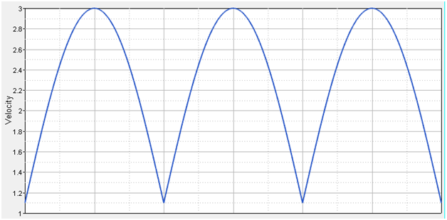
Velocity variation

Note	Multiply `time` with 10, 25 will vary velocity at frequencies 10rad/sec and 25 rad/sec respectively.

mv-7007_motion_panel_properties_tab_example2

7.	Deactivate motion on the Leader Translation Joint created in earlier steps.

Step 8: Simulate model for varying velocities at different frequencies.

1.	Click on the icon to check the model.

2.	Switch to the Run panel by clicking on the Run icon

3.	Under the Main tab, click on the icon to specify the name and location of the MotionSolve .xml file. Save the file with the name Hysteresis_1radpersec.xml in your working directory.

4.	Specify the End time as 3 seconds and the Print Interval as 0.0001 seconds.

mv-7007_run_panel_hypersteresis

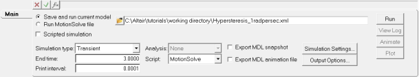
5.	Click on the Run button to run the model.

6.	Modify the velocity expression of the Follower Translation Joint and run the model with the file names and end times specified in the table below:

Frequency	Expression	File name	End Time (sec)
10 rad/sec	`1.1+1.9ABS(sin(PI(10*time)))`	Hysteresis_10radpersec.xml	0.3
25 rad/sec	`1.1+1.9ABS(sin(PI(25*time)))`	Hysteresis_25radpersec.xml	0.12

Step 9: Plotting Hysteresis curves.

1.	Select HyperGraph by clicking in the window.

2.	Load results for the 1 rad/sec frequency.

-	Click on the Open Data File icon .

-	Browse to the working directory and select the Hysteresis_1radpersec.abf file.

mv-7007_build_plots_panel_example

3.	Plot Follower velocity versus Time.

-	Select X-axis Data Type as Time.

-	Select the following for the Y-axis data:

Y Type	Marker Velocity
Y Request	Follower_Velocity- (on Follower)
Y Component	VX

4.	Plot Friction force versus Time.

-	Select X-axis Data Type as Time.

-	Select the following for the Y-axis data:

Y Type	Expression
Y Request	Friction_Force
Y Component	F4

mv-7007_velocity_friction_force_graph

Follower Velocity and Friction Force

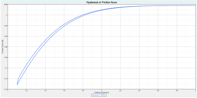
5.	Plotting Friction Hysteresis curve (Friction Force versus Velocity).

There is an initial transition of friction force values, therefore you will plot hysteresis curve excluding first cycle data (in other words, 0 to 1 sec.).

-	Click on the Define Curves icon on the Curves toolbar.

-	Click on the Add button to add a new curve.

mv-7007_build_plots_panel_curve3

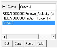
-	Rename Curve3 as 1rad/sec.

mv-7007_build_plots_panel_1rad_sec

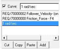
-	For the X and Y data, select the Source type as Math.

mv-7007_build_plots_panel_source_math

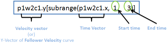
-	Populate X data to select velocity between time interval 1 to 3 secs using the subrange function: p1w2c1.y[subrange(p1w2c1.x,1,3)].

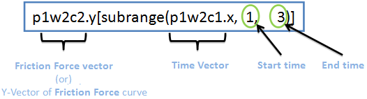
mv-7007_subrange_function_expression_example_mvtut

-	Populate Y data to select Friction force between time interval 1 to 3 secs using the subrange function: p1w2c2.y[subrange(p1w2c1.x,1,3)].

mv-7007_subrange_function_expression_example2_mvtut

-	Click the Apply button.

mv-7007_hysteresis_in_friction_graph

6.	Similarly, plot hysteresis curves for frequencies 10rad/sec (Hysteresis_10radpersec.abf) and 25 rad/sec (Hysteresis_10radpersec.abf) following Steps 3 -5 above.

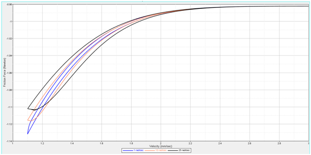
mv-7007_hysteresis_frequency_curves_graph

Hysteresis curves at different frequencies

The velocity variation with higher frequency will have widest hysteresis loop.