Static Ride Analysis

Introduction

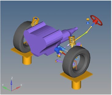
The Static Ride analysis is a simulation of both wheels moving up and down, in phase, with the steering wheel held fixed. The chassis is fixed-to-ground. The displacement of the wheel center is prescribed by the user. The suspension moves via a simple control system and a “suspension test rig”. The wheel is constrained at the tire patch location to the suspension test rig using an in-plane joint. Standard suspension requests (Caster, Camber, Toe, etc.) are included as part of the ride analysis and are described here. The Front and Rear suspension ride analyses are similar.

static_ride_analysis_front_example_mv

Front Suspension Static Ride Analysis

static_ride_analysis_rear_example_mv

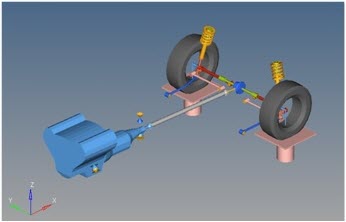
Rear Suspension Static Ride Analysis

Detailed Description

The Static Ride analysis is designed to work with front and rear half vehicle models that have been built through the MotionView Assembly Wizard. The analysis should attach to the model automatically when added through the Task Wizard. The analysis can be used with models built by hand, as long as the attachment scheme in the analysis is strictly followed.

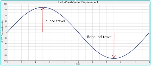
The analysis begins at Zero displacement (design position).

Time (in Seconds)	Action
0 to 2.5	Wheels moves from Design Position to Jounce Position
2.5 to 5.0	Wheels moves from Jounce Position to Design Position
5.0 to 7.5	Wheels moves from Design to Rebound Position
7.5 to 10.0	Wheels moves from Rebound Position to Design Position
10.0	Analysis Ends

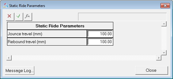
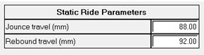
Suspension travel is entered on the Static Ride Parameters form in the analysis. Travel is assumed to be symmetric. The suspension displacement follows a simple harmonic function (sin wave) pattern.

static_ride_analysis_sr_parameters_dialog_mv

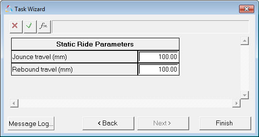
Static Ride Parameters Dialog (Front Half)

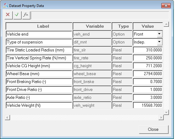
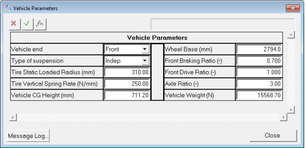
A total of forty-seven outputs are calculated, including all of the Suspension Design Factors. Input data for the SDF’s are entered on the Vehicle Parameters form in the Static Ride analysis (shown below).

static_ride_analysis_vehicle_parameters_dialog_mv

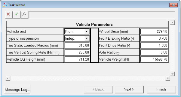
Vehicle Parameters Dialog (Front Half)

How The Analysis Works

The Static Ride analysis is a vertical displacement of the suspension, with the wheels moving in phase. The mechanism to perform this is described below:

•	A Jack body is included in the analysis.

•	The Jack body is constrained to ground with a Translational joint, allowing the Jack body to only move in the vertical direction.

•	An Inplane joint constrains the jack to the wheel at the SLR distance entered in the Vehicle Parameters form.

•	The Solver Variables “Left Command Variable” and “Right Command Variable” define the desired displacement of the Jack bodies.

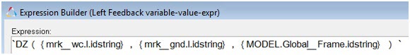
•	The Solver Variables “Left Feedback Variable” and “Right Feedback Variable” measure the distance in the Z direction between the wheel center point on the wheel, and the wheel center point on the ground.

•

Solver Differential Equations “diff left jack” and “diff right jack” are defined as the difference between the Feedback and Command variables. An IF statement and the MODE function is used to turn the Solver Differential Equation on during Statics and Quasi-statics and set it to zero (turning off the Solver Differential Equation) during the remaining analysis modes (Kinematics, Initial Conditions, Dynamics, and Linear Analysis).

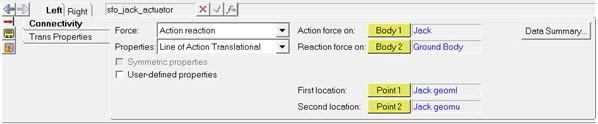
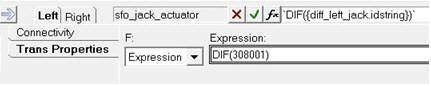
•	A Force “Jack Vertical Actuator” is defined to be the DIF (value) of the Solver Differential Equation “diff left jack” using an expression.

•	The Jack Vertical Actuator force moves the suspension through jounce and rebound. The force magnitude is determined by the Differential Controller value.

Important Notes

The control diff (a simple control system) is used for two reasons:

-	The control system and test rig mechanism does not add constraints to the suspension. This allows the wheel center compliance matrix to be calculated easily, which is used in the suspension design factor calculations.

-	A Force is applied on the test rig “Jack” to move the wheel center vertical (Z) displacement through a prescribed motion. A control system is required for this type of system.

System Description

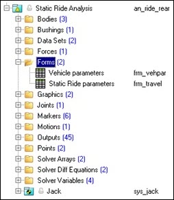
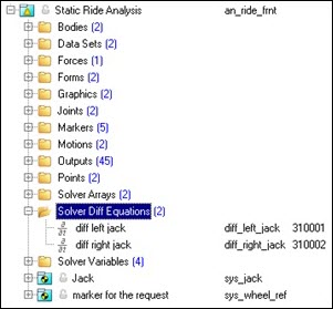
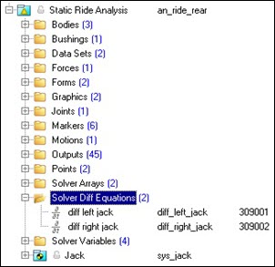
The entities in the analysis are displayed in the MotionView Project Browser as shown in the image below:

static_ride_analysis_front_prjct_brwsr_example_mv

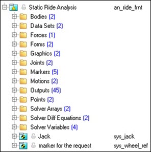
Project Browser View - Front Half - Static Ride Analysis

static_ride_analysis_rear_prjct_brwsr_example_mv

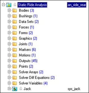
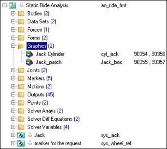
Project Browser View - Rear Half - Static Ride Analysis

Nine types of modeling element containers are used to define the analysis. One sub-system (a Drive torque controller) is also included in the analysis.

Thirteen modeling element types are used in the front analysis and fourteen modeling element types are used in the rear suspension analysis (see below). The sub systems “Jack” and “Marker for Request” are also described below.

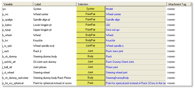
The analysis uses the standard analysis attachment. The attachments resolve automatically if the model is built through the Model Wizard. The attachments contain the minimum data the analysis needs to run the analysis. The attachments are standard for most analyses.

static_ride_analysis_front_attachements_example_mv

Front Half Static Ride Analysis - Attachments

static_ride_analysis_rear_attachements_example_mv

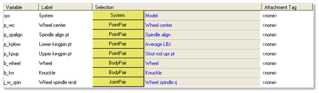
Rear Half Static Ride Analysis - Attachments

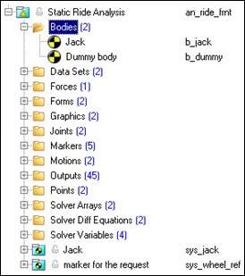
Two bodies are used in the Front Half Static Ride analysis, “Jack” and “Dummy body”. The “Jack” is used to simulate a platform moving vertically to displace the suspension. The "Dummy body" is included in the analysis to make the system compatible with ADAMS modeling. The "Dummy body" is attached to the knuckle with a fixed joint and has no role in the analysis when it is run in MotionSolve.

static_ride_analysis_front_bodies_prjct_brwsr_example_mv

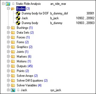
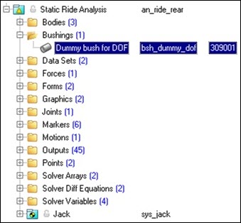
Project Browser View - Bodies - Front Half Static Ride Analysis

The Rear suspension analysis is shown below. The “Dummy body for DOF” body is included to make the Degrees of Freedom work out for certain suspensions. The Dummy body is constrained to ground with a soft bushing.

static_ride_analysis_rear_bodies_prjct_brwsr_example_mv

Project Browser View - Bodies - Rear Half Static Ride Analysis

There are no bushings in the Front suspension analysis. One bushing is included in the Rear Half suspension analysis, “Dummy bush for DOF”. The ‘Dummy bush for DOF” constrains the “Dummy Body for DOF” body to ground with a soft bushing rate. The bushing is used to make the Degrees of Freedom work properly for certain models.

static_ride_analysis_rear_bushings_prjct_brwsr_example_mv

Project Browser View - Bushings - Rear Half Static Ride Analysis

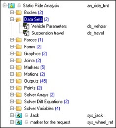
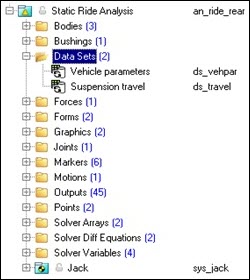
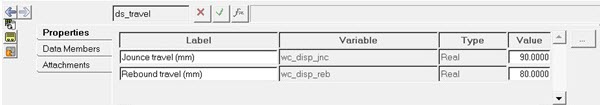
Two datasets are used in the system, "Vehicle Parameters" and "Suspension travel". The "Suspension travel" dataset is used to store the suspension travel inputs for jounce and rebound. Edit the parameters on the “Suspension travel” form. The "Vehicle Parameters" dataset is used to store data used to calculate the Suspension Design Factors. Edit the input values on the “Vehicle Parameters” form. The input values, and their use is described in depth in the Suspension Design Factors section.

static_ride_analysis_front_datasets_prjct_brwsr_example_mv

Project Browser View - Datasets - Front Half Static Ride Analysis

static_ride_analysis_rear_datasets_prjct_brwsr_example_mv

Project Browser View - Datasets - Rear Half Static Ride Analysis

static_ride_analysis_dataset_prop_data_dialog_mv

Dataset Property Dialog - Datasets "Vehicle Parameters"

static_ride_analysis_dataset_prop_data_dialog2_mv

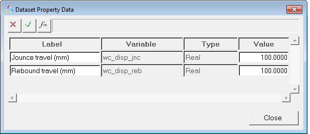
Dataset Property Dialog - Datasets "Suspension Travel"

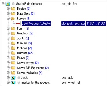
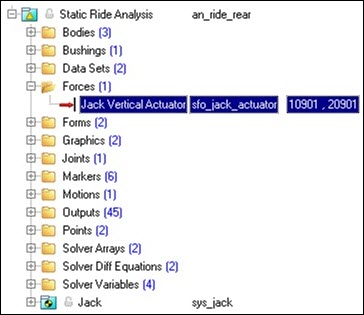
The Front and Rear Static Ride analyses include one force pair, the “Jack Vertical Actuator”. This force applies a vertical force on the jack which moves the suspension into jounce and rebound. The Force is controlled by a DIF statement. The browser view of the force is shown below:

static_ride_analysis_front_forces_prjct_brwsr_example_mv

Project Browser View - Force - Front Half Static Ride Analysis

static_ride_analysis_rear_forces_prjct_brwsr_example_mv

Project Browser View - Force - Rear Half Static Ride Analysis

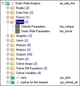
Two Forms are included in the Static Ride Analysis. These Forms are used to modify the inputs into the analysis. The “Vehicle Parameters” form is used to edit the inputs used to calculate the Suspension Design Factors. The Suspension Design Factors are described in detail in here. The “Static Ride Parameters” are the jounce and rebound travels used in the analysis. Modify the values to match the desired Wheel Center vertical travel in your suspension. The front and rear forms are the same.

static_ride_analysis_front_forms_prjct_brwsr_example_mv

Project Browser View - Forms - Front Half Static Ride Analysis

static_ride_analysis_rear_forms_prjct_brwsr_example_mv

Project Browser View - Forms - Rear Half Static Ride Analysis

static_ride_analysis_front_forms_vehicle_parameters_dialog_mv

Vehicle Parameters Dialog - Forms - Front Half Static Ride Analysis

static_ride_analysis_front_forms_static_ride_parameters_dialog_mv

Static Ride Parameters Dialog - Forms - Front Half Static Ride Analysis

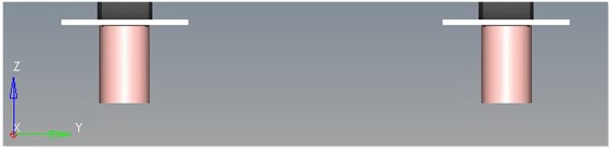
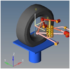
Two Graphics are defined in the Front and Rear Static Ride Analysis, “Jack Cylinder” and “Jack Patch”. The graphics represent test apparatus used to exercise the front suspension.

static_ride_analysis_front_graphics_prjct_brwsr_example_mv

Project Browser View - Graphics - Front Half Static Ride Analysis

static_ride_analysis_jack_graphics_example_mv

Jack Graphics Example

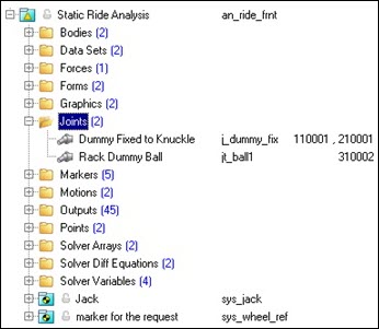
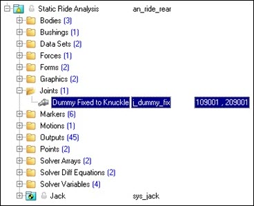
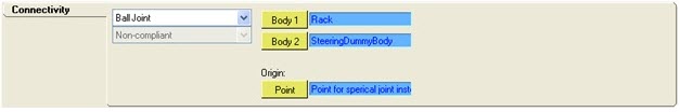
Two joints, “Dummy Fixed to Knuckle” and “Rack Dummy Ball” joints are included in the Front Half Static Ride analysis; one joint, “Dummy Fixed to Knuckle” is included in the Rear Half Static Ride analysis. "Dummy Fixed to Knuckle" is a fixed joint which attaches the Knuckle to the Dummy body. The dummy joints are included to constrain dummy bodies. The dummy bodies are used to make certain analyses work with ADAMS.

static_ride_analysis_front_joints_prjct_brwsr_example_mv

Project Browser View - Joints - Front Half Static Ride Analysis

static_ride_analysis_rear_joints_prjct_brwsr_example_mv

Project Browser View - Joints - Rear Half Static Ride Analysis

static_ride_analysis_joints_panel_dummy_example_mv

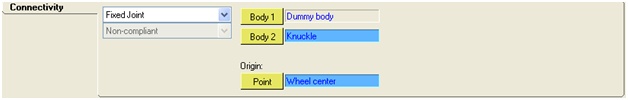
Joints Panel - Dummy Fixed to Knuckle Joint - Front Half Static Ride Analysis

static_ride_analysis_joints_panel_rack_dummy_example_mv

Joints Panel - Rack Dummy Ball Joint - Front Half Static Ride Analysis

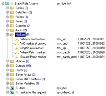
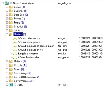
Five markers are included in the Front Half Static Ride; six markers are used in Rear Half Static Ride analysis. The markers are described in the tables located below:

Front Suspension Markers

Marker Label	Marker Varname	Description	Use
Wheel Center	mrk_wc	Marker Pair on the “Dummy Body” at the Wheel center, Z axis pointing inboard, ZX plane of the marker along global X.	The primary Wheel Center Marker Pair, used in the system that actuates the suspension motion and used to calculate the SDF’s in the SDF subroutine.
WC marker at Ground	mrk_gnd	Marker pair on “Ground” at the Wheel Center; Z axis along global Z and ZX plane along global X.	Used in the system that actuates the suspension motion and used to calculate SDF’s in the SDF subroutine.
Kingpin Axis Marker	mrk_kp	Marker Pair on the knuckle, at the LBJ or estimated LBJ location, with a Z axis pointing at the actual or estimated UBJ location.	Used to calculate the vehicle kingpin metrics in both a user output request and in the SDF subroutine. The marker Z axis is used for the calculations.
Wheel Patch marker	mrk_patch	Marker Pair on the Wheel at the tire patch location. The tire patch location is calculated using the SLR entered on the Vehicle Parameters form, and is the “Jack GeomU” point. The marker Z axis is along global Z and the marker X axis is in the global ZX plane.	Used to calculate the Roll angle/Track width in the Roll Angle/Track Width user defined expression output.
Ground Patch Marker	mrk_patch_grnd	Marker Pair on body “ground” at the tire patch location. The tire patch location is calculated using the SLR entered on the Vehicle Parameters form, and is the “Jack GeomU” point. The marker Z axis is along the global Y (lateral) axis and the marker X axis is in the global X plane.	Not currently used in the MotionSolve analysis.

Rear Suspension Markers

Marker Label	Marker Varname	Description	Use
Wheel Center Marker	mrk_wc	Marker Pair on the “Dummy Body” at the Wheel center, Z axis pointing inboard, ZX plane of the marker along global X.	The primary Wheel Center Marker Pair, used in the system that actuates the suspension motion and used to calculate the SDF’s in the SDF subroutine.
WC marker at Ground	mrk_gnd	Marker pair on “Ground” at the Wheel Center; Z axis along global Z and ZX plane along global X.	Used in the system that actuates the suspension motion and used to calculate SDF’s in the SDF subroutine
Ground Reference at contact patch	Tcp_grnd	Marker pair on body “ground” at the Jack Geomu point (tire patch). The marker Z axis is along the global Z and the XZ plane of the marker is along the global X axis.	This Marker is not used in the MotionSolve analysis
Ground Reference at wc	wc_grnd	Marker Pair on ground at the wheel center location. The marker Z axis is along global Z and the marker X axis is in the global ZX plane.	This marker is not used in the current MotionSolve analysis.
Kingpin Axis Marker	mrk_kp	Marker Pair on the knuckle, at the Lower Ball Joint or estimated Lower Ball Joint location, with a Z axis pointing at the actual or estimated Upper Ball Joint location. In strut type suspensions the marker Z axis points at the top of the strut.	Used to calculate the vehicle kingpin metrics in both a user output request and in the SDF subroutine. The marker Z axis is used for the calculations.
Wheel Patch marker	mrk_patch	Marker Pair on body “ground” at the Jack geomu point (tire patch). The marker Z axis is along the global Z (lateral) axis and the marker ZX plane axis is in the global X plane.	Not currently used in the MotionSolve analysis.

static_ride_analysis_front_markers_prjct_brwsr_example_mv

Project Browser View - Markers - Front Half Static Ride Analysis

static_ride_analysis_rear_markers_prjct_brwsr_example_mv

Project Browser View - Markers - Rear Half Static Ride Analysis

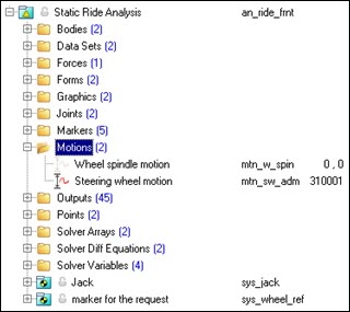
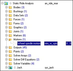
Two motions are included in the Front Half Static Ride analysis, and a single motion is included in the Rear Half Static Ride analysis. The “Wheel spindle motion” is used in both front and rear, and the “Steering wheel motion” is used in front analysis. The "Wheel spindle motion" fixes the wheel to the knuckle to prevent wheel rotation. The "Steering wheel motion" is used to hold the steering wheel during most analyses, and is used to turn the steering wheel during a steering analysis. The "Wheel spindle motion" is deactivated and not used in both the front and rear ride analyses.

static_ride_analysis_front_motions_prjct_brwsr_example_mv

Project Browser View - Motions - Front Half Static Ride Analysis

static_ride_analysis_rear_motions_prjct_brwsr_example_mv

Project Browser View - Motions - Rear Half Static Ride Analysis

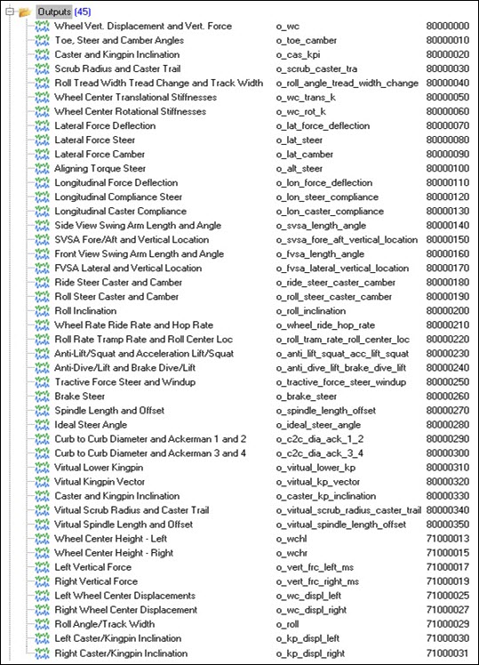
Forty Five Outputs are included in both Front and Rear Static Ride analyses.

static_ride_analysis_front_outputs_prjct_brwsr_example_mv

Project Browser View - Outputs - Front and Rear Half Static Ride Analysis

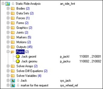
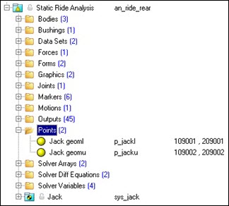
Two point pairs are defined in the Front and Rear Half Static Ride analyses. The points are used to create the Jack graphics and are referred to by the analysis markers. The points contain parametric logic to define their X, Y, and Z locations. No user modification of any points should be necessary. The point pairs for both the Front and Rear analyses are described in the table below:

Point	Description	Use
Jack GeomL (Jack Geometry Lower)	A point 320 mm below the Jack GeomU point.	Used to define the Jack Geometry. The 320 mm is an arbitrary number.
Jack Geomu (Jack Geometry Upper)	An estimate of the tire patch location, calculated using the Wheel Center location, the spindle axis , and the SLR entered in the Vehicle Parameters form.	Used in SDF calcs and as the location to transfer load from the test rig platen to the wheel.

static_ride_analysis_front_points_prjct_brwsr_example_mv

Project Browser View - Points - Front Half Static Ride Analysis

static_ride_analysis_rear_points_prjct_brwsr_example_mv

Project Browser View - Points - Rear Half Static Ride Analysis

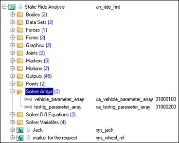
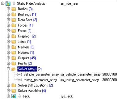
There are two solver arrays in the Front and Rear Half Static Ride analyses; "Vehicle parameter array" and "Testrig parameter array". The "Vehicle parameter array" contains vehicle information that is used to calculate the SDF’s. Some of the data is also used in the analysis to create point locations and forces. The data is entered in the Vehicle Parameter Form. The "Testrig parameter array" contains point, force and motion data, and is passed to the SDF subroutine and used to run the SDF calculation analysis. The "Testrig parameter array" is symbolically defined and should not require editing.

Vehicle Parameter Array	Description	Use
Ds_vehpar.veh_end.ival	Vehicle End: 1=front suspension; 2=rear suspension; 3=2nd rear suspension	Communicates the suspension type to the SDF subroutine. The subroutine calculates different values for certain parameters depending on which end of the vehicle is being analyzed.
Ds_vehpar.dif_mnt.ival	Differential Mount type 0=mounted to body 1=Unsprung mount (integral with the axle)	Used in the SDF calculations in the anti-lift and anti-dive calculations.
Ds_vehpar.tire_slr.value	Tire Static Loaded Radius in mm	Used to locate the “Jack GeomU” point and in many of the SDF calculations.
Ds_vehpar.tire_rate.value	Tire Spring Rate in N/mm	Used in the SDF calculations
Ds_vehpar.cg_height.value	Vehicle CG height, measured from ground to the CG in the Z direction (mm)	Used in the SDF calculations (especially the Anti-lift and anti-dive calculations)
Ds_vehpar.wheel_base.value	Vehicle Wheelbase (mm)	Used in the SDF calculations (especially the Anti-lift and anti-dive calculations)
Ds_vehpar.front_brake.value	The Ratio of front brake torque to total brake torque (typically .6 to .7).	Used in the SDF calculations (especially the Anti-lift and anti-dive calculations)
Ds_vehpar.front_drive.value	The ratio of the engine torque applied to the front axle divided by total torque.	Used in the SDF calculations (especially the Anti-lift and anti-dive calculations)
Ds_vehpar.axle_ratio	The nominal Axle ratio of the suspension being analyzed. Typically in the 2.7-5.0 range.	Used in the SDF calculations (especially the Anti-lift and anti-dive calculations)
Ds_vehpar.veh_weight.value	Total Vehicle Mass in Kg	Used in SDF calculations and in the vehicle load analysis ev

Testrig Parameter Array

The Testrig array is populated by the analysis using the symbolic logic provided by MotionView and should not require editing. The Testrig parameters are defined in the table below:

Parameter name	Description	Use
mrk_wc.l.id	Left Wheel Center Marker ID-Marker at the Left Wheel Center; Z axis points inboard along the spindle axis; ZX marker plane is along Global X; the resulting marker Y axis is down.	The primary point location for left suspension SDF calculations. Most geometric properties and most Compliant SDF parameters are calculated using this point as input.
mrk_wc.r.id	Right Wheel center Marker ID-Marker at the Right Wheel Center; the marker Z axis points inboard along the spindle axis; the marker ZX plane is along global X; The resulting marker Y axis is up.	The primary point location for right suspension SDF calculations. Most geometric properties and most Compliant SDF parameters are calculated using this point as input.
mrk_kp.l.id	Left Kingpin Axis Marker ID- The marker placed at the Left Lower Ball Joint or a location that defines a point on the Left Kingpin axis. The Z axis of the marker points to the Left Upper Ball Joint or a point that defines a point on the kingpin axis.	Marker Z axis is used for Caster and Kingpin Inclination calculations for the left side of the vehicle.
mrk_kp.r.id	Right Kingpin Axis Marker ID- The marker placed at the Right Lower Ball Joint or a location that defines a point on the Right Kingpin axis. The Z axis of the marker points to the Right Upper Ball Joint or a point that defines a point on the kingpin axis.	Marker Z axis is used for Caster and Kingpin Inclination calculations for the right side of the vehicle.
mrk_gnd.l.id	The ID of the Left Wheel Center Marker on body “ground”. The Marker is on the ground body at the Left Wheel Center location. The marker Z axis is parallel to the Global Z axis and the marker X axis is parallel to the global X axis.	Marker is used for the left Wheel displacement control system and left wheel center displacement calculations in the SDF routine.
mrk_gnd.r.id	The ID of the Right Wheel Center Marker on body “ground”. The Marker is on the ground body at the Right Wheel Center location. The marker Z axis is parallel to the Global Z axis and the marker X axis is parallel to the global X axis.	Marker is used for the right Wheel displacement control system and right wheel center displacement calculations in the SDF routine.
sfo_jack_actuator.l.i.id	I Marker ID of the Left Force between the Jack and ground that is used to actuate the left wheel suspension motion.	Forces are used for the SDF subroutine calculations and the force reported by the SDF routine. The I and J marker ID’s are required to recover the correct force.
sfo_jack_actualtor.r.i.id	J Marker ID of the Left Force between the Jack and ground that is used to actuate the Left wheel suspension motion.	Forces are used for the SDF subroutine calculations and the force reported by the SDF routine. The I and J marker ID’s are required to recover the correct force.
sfo_jack_actuator.j.i.id	I Marker ID of the Right Force between the Jack and ground that is used to actuate the left wheel suspension motion.	Forces are used for the SDF subroutine calculations and the force reported by the SDF routine. The I and J marker ID’s are required to recover the correct force.
sfo_jack_actualtor.j.i.id	J Marker ID of the Right Force between the Jack and ground that is used to actuate the Right wheel suspension motion.	Forces are used for the SDF subroutine calculations and the force reported by the SDF routine. The I and J marker ID’s are required to recover the correct force.
b_str_dummy.cm.id	Steering Dummy Body Center of Mass ID number. The Center of mass marker for the dummy body attached to the steering rack.	Not used by the current subroutine but kept in the software to maintain compatibility with ADAMS simulations.

static_ride_analysis_testrig_parameter_array_example_mv

static_ride_analysis_rear_example2_mv

static_ride_analysis_front_solver_array_prjct_brwsr_example_mv

Project Browser View - Solver Array - Front Half Static Ride Analysis

static_ride_analysis_rear_solver_array_prjct_brwsr_example_mv

Project Browser View - Solver Array - Rear Half Static Ride Analysis

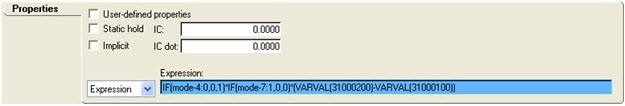
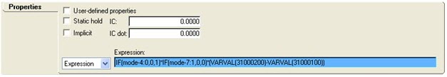
The Front and Rear Half Static Ride include two solver differential equations, Differential left jack and Differential right jack. The Solver Differential Equations are part of the control system used to move the suspension through the requested travel. The Solver Differential Equations are similar for both the front and rear suspensions.

The front left equation is as follows:

IF(mode-4:0,0,1)*IF(mode-7:1,0,0)*(VARVAL(31000200)-VARVAL(31000100))

A break down of the equation is provided below:

IF(mode-4:0,0,1)	When mode (the solution type of the solver) is less than or equal to 4 the expression evaluates to Zero. When Mode is greater than 4, the expression evaluates to one.
IF(mode-7:1,0,0)	When mode (the solution type of the solver) is less than or equal to 7 the expression evaluates to One. When Mode is 7 or greater, the expression evaluates to zero.
VARVAL(31000200)	The Solver Variable value that represents the “commanded” displacement of the left wheel center Z displacement.
VARVAL(31000100)	The Solver Variable value that represents the actual displacement of the left wheel center in the global Z direction from the “design” position.

As a result:

IF(mode-4:0,0,1)*IF(mode-7:1,0,0)	This expression is One for Modes 5 and 6, which are statics and quasistatics. For all other modes this evaluates to zero. This effectively turns the Solver Differential Equation off for solution sequences other than statics and Quasistatics.
VARVAL(31000200)-VARVAL(31000100))	The commanded displacement minus the actual displacement. If the suspension is following the commanded value this will be zero.

The Solver Differential Equation maintains the wheel displacement due to the following property of Solver Differential Equations: For static and quasi-static solutions, the derivative of the dynamic state is set to zero. This converts the Control_Diff to an algebraic equation for these two analyses. See the Control_Diff topic in the MotionSolve Reference Guide for additional information.

static_ride_analysis_front_solver_diff_equat_prjct_brwsr_example_mv

Project Browser View - Solver Differential Equations - Front Half Static Ride Analysis

static_ride_analysis_rear_solver_diff_equat_prjct_brwsr_example_mv

Project Browser View - Solver Differential Equations - Rear Half Static Ride Analysis

static_ride_analysis_front_solver_diff_equat_panel_example_mv

Panel View - Solver Differential Equations - Front Half Diff Left Jack

static_ride_analysis_rear_solver_diff_equat_panel_example_mv

Panel View - Solver Differential Equations - Front Half Diff Right Jack

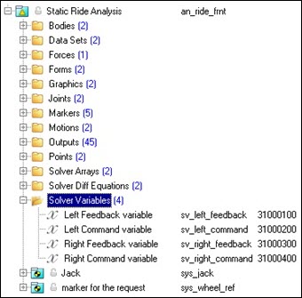
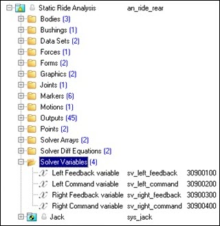
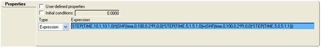
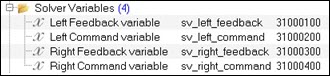
The Static Ride analysis consists of four solver variables:

•	Left Feedback variable

•	Left Command variable

•	Right Feedback variable

•	Right command variable

Solver variables are part of the wheel displacement control system. Each Solver variable is described in the table below:

Variable Name	Description
Left Feedback Variable	Global Z Displacement of the left wheel center marker, relative to the original location of the left Wheel center, in the global coordinate system.
Left Command Variable	Requested Displacement of the left Wheel center. From 0-5 seconds a half sin function with a magnitude equal to the “Jounce” travel defined on the “static ride parameters” form. From 5-10 seconds a half sin function with a magnitude equal to the “Rebound” travel defined on the “static ride parameters” form.
Right Feedback Variable	Global Z Displacement of the right wheel center marker, relative to the original location of the right Wheel center, in the global coordinate system.
Right Command Variable	Requested Displacement of the right Wheel center. From 0-5 seconds a half sin function with a magnitude equal to the “Jounce” travel defined on the “static ride parameters” form. From 5-10 seconds a half sin function with a magnitude equal to the “Rebound” travel defined on the “static ride parameters” form.

static_ride_analysis_solver_variables_example_mv

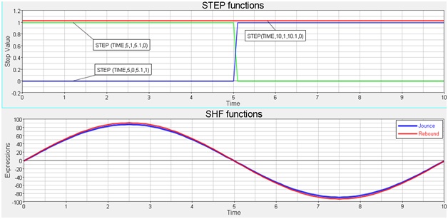
Plot of the Left WC Command Variable vs. Time

static_ride_analysis_front_solver_variables_prjct_brwsr_example_mv

Project Browser View - Solver Variables - Front Half Static Ride Analysis

static_ride_analysis_rear_solver_variables_prjct_brwsr_example_mv

Project Browser View - Solver Variables - Rear Half Static Ride Analysis

static_ride_analysis_front_solver_variable_panel_example_mv

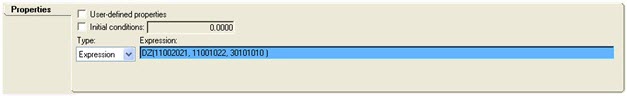
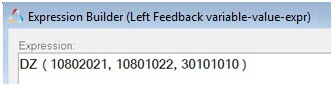
Panel – Solver Variable - Front Half Left Feedback Variable

static_ride_analysis_front_solver_variable_panel_comm_var_example_mv

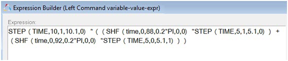
Panel – Solver Variable - Front Half Left Command Variable

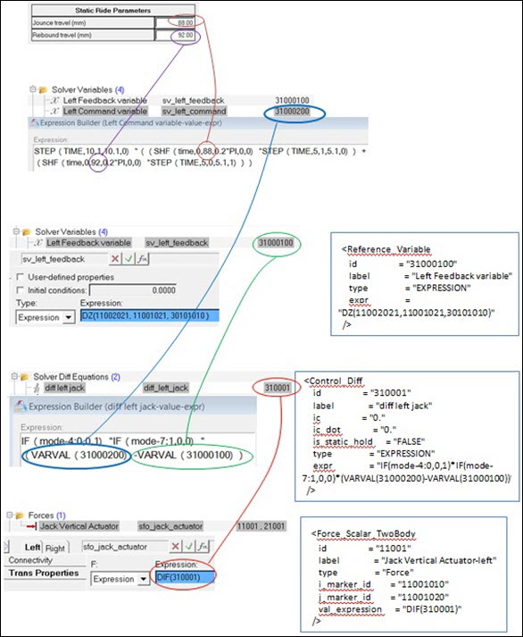
Many of the half car analyses use a control system to displace the wheels in Jounce and Rebound. The system applies a Force on the Jack to move the wheel center through a displacement defined by the “Left Command Variable” and “Right Command variable”. The control system only works while running Statics and Quasi-statics solutions.

A diagram of the system is shown below. The solver statements that are written for some MotionView entities are shown in the diagram. The system is symmetric, and the front and rear suspensions use a similar scheme.

static_ride_analysis_whl_displ_cntrl_sys_example_mv

A description of the system is as follows (from top to bottom of the diagram):

•	Jounce Travel and rebound Travel are entered in the “Static Ride Parameters” form. Travel is assumed to be symmetric.

•	The Solver variables “left command variable” (shown) and the “right command variable” (not shown) refer to the Travels from the “Static Ride Parameters” form.

•

The equations in the “left command variable” and “right command variable” Solver variables create a sin wave which has a positive peak at 2.5 seconds with a magnitude equal to the jounce travel, and a negative minimum at 7.5 seconds at the “rebound travel” magnitude. The solver equation is further explained in the “Solver Variables” section below.

•	The Solver Variables “Left Feedback variable” and “Right Feedback variable” are defined. The variable is the displacement of the wheel center on the wheel, relative to the original wheel center position, in the global Z direction.

•

The Solver Differential Equation is defined (for left and right side) to be the difference between the command variable and the actual variable. If the Wheel Center displacement follows the command variable, the Differential Equation will be zero. The Differential Equation is set to zero for solution e=sequences other than “Statics” and “quasi-statics” using IF statements and the MODE variable.

•	A force is defined that is equal to the Control Differential of the wheel.

•

The Solver Differential Equation maintains the wheel displacement due to the following property of Solver Differential Equations: “For static and quasi-static solutions, the derivative of the dynamic state is set to zero. This converts the Control_Diff to an algebraic equation for these two analyses.”

Element Description

A detailed description of the elements included in the Wheel Control System are provided below:

The Wheel Control system form is shown below. The “Static Ride Parameters” form contains the Jounce and rebound travel that are applied to the suspension system. Travel is symmetric (L<->R). The Jounce and Rebound variables are defined in the “Suspension Travel” Dataset. Dataset types and variable names are defined in the dataset; data is normally entered on the form.

static_ride_analysis_whl_cntrl_sys_sr_paramaters_example_mv

Static Ride Parameters

static_ride_analysis_whl_cntrl_sys_susp_trvl_panel_example_mv

Suspension Travel dataset

Four Solver Variables are defined; Left and Right Feedback and Left and Right Command variables. The Command variables contain equations that define the wheel center displacement with respect to time. The feedback variables measure the Wheel Center displacement. The left and right sides are symmetric so only the left side solver variables are described below:

static_ride_analysis_whl_displ_cntrl_solver_variables_prjct_brwsr_example_mv

Left Command Variable

static_ride_analysis_whl_displ_cntrl_solver_variables_expr_builder_example_mv

Equation	Description
STEP(TIME,10,1,10.1,0)	A step function that is one when Time is less than 10 and zero when time is greater than 10. This makes the entire equation evaluate to zero after T=10.
SHF(time,0,88,0.2*PI,0,0)	A Simple Harmonic Function, Time based, Time offset of zero, magnitude of 88, Frequency=.2*pi, with zero phase shift and a zero average value.
STEP(TIME,5,1,5.1,0)	A step function that is one when Time is less than 5 and Zero when Time is greater than 5.1. This turns the Jounce SHF off when T>5.1.
SHF(TIME,0,92,0.2*pi,0,0)	A Simple Harmonic Function, Time based, Time offset of zero, magnitude of 92, Frequency=.2*pi, with zero phase shift and a zero average value.
STEP(TIME,5,0,5.1,1)	A step function that is 0 when Time is less than 5 and One when Time is greater than 5.1. This turns the Rebound SHF on when T>5.1.

The functions are plotted below:

static_ride_analysis_solver_variables_plotting_example_mv

Step and SHF functions in the Solver variable Command variable

static_ride_analysis_solver_variables_graphic_example_mv

Resulting “Left Command variable” vs Time

The Solver Variable “Left Feedback variable” is shown below. The Feedback variable gives the Displacement of the wheel center marker on the Wheel body, relative to the initial location of the wheel, in the global coordinate frame. The right Feedback variable is similar.

static_ride_analysis_slvr_fdbck_var_expr_builder_example_mv

Symbolically the expression is:

static_ride_analysis_slvr_fdbck_var_expr_builder_example2_mv

The Markers are described in the table below:

Marker Number	Marker Symbol	Description
10802021	Mrk_wc.l.idstring	Marker on the wheel at the wheel center.
10801022	Mrk_gnd.l.idstring	A marker on ground at the wheel center.
30101010	MODEL.Global_Frame.idstring	A marker on ground at the Global Origin, with the same orientation as the Global coordinate frame.

The Solver Differential Equations are two equations (left & right wheel) that define a differential equation to control the wheel displacement. The equation is of the form f(x)=Dcommand-Dactual, and is modified by mode statements to equal zero for simulation modes other than statics and quasi-statics. The equation is a key to the control system used to move the wheels.

static_ride_analysis_whl_displ_cntrl_solver_diff_equ_prjct_brwsr_example_mv

static_ride_analysis_whl_displ_cntrl_solver_diff_equ_expr_bldr2_example_mv

Symbolically the expression is:

static_ride_analysis_whl_displ_cntrl_solver_diff_equ_expr_bldr_example_mv

The expression shown above uses the “mode” and “if” functions from Motionsolve, along with the VARVAL function. The combination of the two IF statements create logic that makes the DIF equal zero for all modes except statics and quasi-statics. The logic is shown in the "truth" table developed below:

Mode	Mode Value	Mode-4	IF(mode-4:0,0,1)	Mode-7	IF(mode-7:1,0,0)	IF(mode-4:0,0,1) *IF(mode-7:1,0,0)
Kinematics	1	-3	0	-6	1	0
Reserved	2	-2	0	-5	1	0
Initial Conditions	3	-1	0	-4	1	0
Dynamics	4	0	0	-3	1	0
Statics	5	1	1	-2	1	1
Quasi Statics	6	2	1	-1	1	1
Linear Analysis	7	3	1	0	0	0

The function (VARVAL(30800200)-VARVAL(30800100)) is the difference between the command variable and the measured variable. If the command is following the measured, this expression should equal zero.

The actuator Force Pair is shown below. The left side is shown and the right side behaves in the same manner. The force acts on the jack and is reacted on ground. The force acts in the vertical direction. The force is set to the DIF(308001) magnitude. When the DIF is evaluated during statics and quasi-statics, the derivative of the Solver Differential Equation is set to zero. The result is that a Force is generated by the DIF that forces the measured wheel displacement to follow the command wheel displacement.

static_ride_analysis_actuator_force_panel_example_mv

static_ride_analysis_actuator_force_panel_trans_prop_example_mv

How The Wheel Control System Works

The wheel control system works as follows:

•	The prescribed wheel displacements for left and right wheel center Z displacement are defined by the expressions in the solver variables “Left Command value” and “Right Command value”.

•	The force required to maintain the wheel displacement is defined by the Force pair “Jack vertical Actuator” and is a pure Z force on the “Jack” body on each side of the vehicle. This is set equal to the DIF value.

•	The actual wheel displacements in the Z direction are defined by the solver variables “Left Feedback variable” and “Right Feedback variable”.

•	The controls are defined in the Solver Diff Equations “diff left jack” and “diff right jack” and are the command solver variable minus the feedback solver variable. This will equal zero if the wheel is following the command input

•	The solver treats the Solver Differential equation as an algebraic equation in statics and quasi-statics mode. As a result the DIF value is the force required to maintain the commanded wheel position.

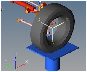
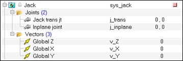
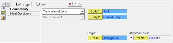
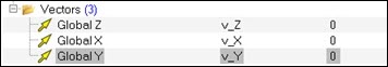
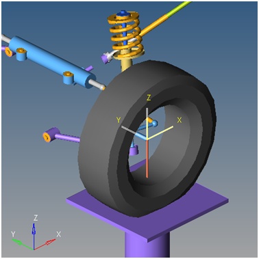
The Jack has two joints and three vectors in it. The joints connect the jack to ground and to the wheel. The vectors are parallel to the Global axes and are used as reference vectors. The graphics of the Jack are in the analysis template, which in this case is the ride analysis.

static_ride_analysis_jack_sys_prjct_brwsr_example_mv

Figure-Jack system Modeling Entities

There are two joint pairs in the Jack system. The first joint is the “Jack Trans jt” which connects the Jack body to ground with a translational joint at the lower end of the jack body. The joint is oriented in the Z (vertical) direction. The joint forces the Jack to travel only in the vertical direction.

static_ride_analysis_jack_system_joints_panel_example_mv

Three vectors are defined along the Global X,Y, and Z axes, and are used to orient certain joints in the model.

static_ride_analysis_jack_sys_vectors_prjct_brwsr_example_mv

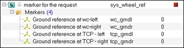
The “Marker for the request” system contains four markers that are used for output requests. The markers are at the wheel center and at the Tirepatch (GeomU) for the Left and Right wheels. All markers are on ground and are oriented to be parallel to the global coordinate frame. The markers are used to measure wheel center or tirepatch travel in output requests.

static_ride_analysis_mrkr_fr_the_rqst_prjct_brwsr_example_mv

static_ride_analysis_mrkr_fr_the_rqst_example_mv

Left Wheelcenter Marker