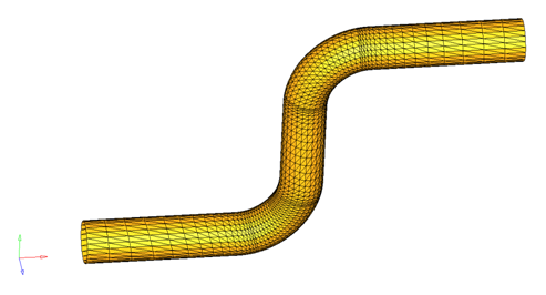
This exercise will cover how to take results from a CFD analysis and apply them to a new model for heat transfer or structural analysis. Using the linear interpolation tools within Engineering Solutions, results from a CFD analysis can be transferred to be loads in an analysis to be run in OptiStruct or any other supported solver.
Typically, scalar results such as temperatures or pressures are mapped. Results must be in a Tecplot file (*.tpl or *.dat). This exercise will demonstrate how Engineering Solutions has a very easy and straightforward way to transfer loads from CFD to a heat transfer of structural analysis.
The model file used in this exercise can be found in the es.zip file. Copy the file(s) from this directory to your working directory.
| 1. | From the menu bar, select Preferences > User Profiles or click  on the Standard toolbar. on the Standard toolbar. |
| 2. | Select Engineering Solutions > CFD > AcuSolve. |
|
| 1. | Click the Open Model icon  on the Standard toolbar. on the Standard toolbar. |
| 2. | Select the s_bend_tube.hm file. |
| 4. | Use the Model browser to turn off the display of the component cube. |
|
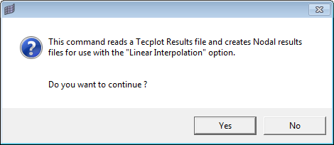
| 1. | From the menu bar, select Tools > Mapping CFD Loads. |
| 2. | This opens a dialog explaining the mapping process and asking if you want to continue. Select Yes. |
| 3. | Browse and select the file Sbend_Model_CFDpp_Tecplot_SURFTEC.DAT. |
| 4. | Select Open to open the file. |
| 5. | This opens the file and creates nodal results files for each result type present in the file. |
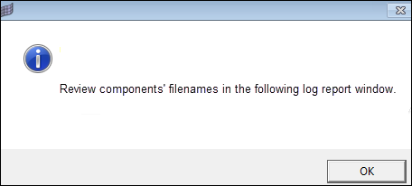
| 6. | Another dialog appears telling you that the file names can be reviewed in the log report window. Click OK to close the window. |
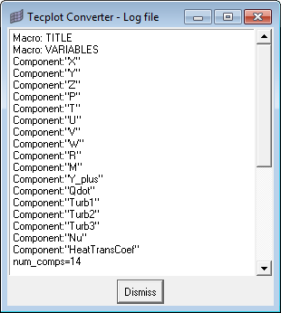
| 7. | Review the log file. Notice that for each scalar data type available in the Tecplot file, a new file was created. The file name is appended with the name of the scalar and “_for_LI”. When you have finished reviewing the file, click Dismiss. |
|
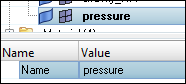
| 1. | Right-click in the Model browser and select Create > Load Collector. The Entity Editor opens. |
| 2. | For Name enter pressure. |
|
| 1. | From the menu bar, click Tools>Linear interpolation>Pressure. |
| 2. | Select elems>by collector and then select the component Tube_Sbend. Click select to accept the selection. |
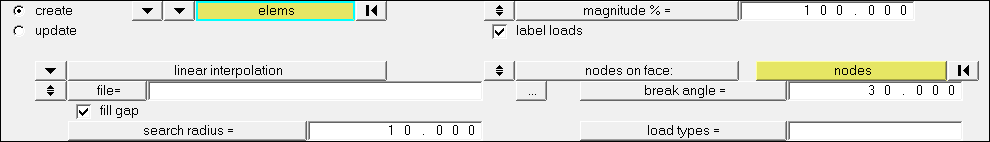
| 3. | Click the switch next to magnitude and select linear interpolation. |
| 4. | There is now a file= field under linear interpolation. Click … next to the file= field to select a file. |
| 5. | Browse for the file Sbend_Model_CFDpp_Tecplot_SURFTEC_P_for_LI.DAT. Click Open. This file contains the pressure results from the CFD analysis. |
| 6. | For search radius, enter 0.05. The search radius is a search distance to find the loads which are within that distance from a centroid or node on which a load is being interpolated. HyperMesh uses the nearest three loads located within that distance to create the load at the centroid or node by linear interpolation. Linear interpolation uses a triangulation method, so if it finds fewer than three loads within that distance no interpolation takes place. While reading the initial loads from a file, if linear interpolation is not possible because the search radius is too small, the original loads are simply applied to the nearest centroid or node. |
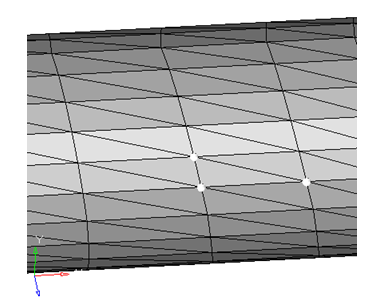
| 7. | Next to nodes on face, click nodes and then select three nodes that define an element (see image below). |
| 9. | Select return to exit the panel. |
|
| 1. | Within the Model browser, expand the Load Collector folder. |
| 2. | To turn off the display of the load collector pressure, click the mesh icon,  , to the left of pressure. The icon will be grayed out and the pressure loads will no longer be displayed. , to the left of pressure. The icon will be grayed out and the pressure loads will no longer be displayed. |
| 3. | Select Tools > Contour Loads. This opens a new tab called Contour Loads. |
| 4. | Click pressure to select the load collector to be contoured. |
| 5. | Click on Accept. This displays the Contour panel and automatically loads the appropriate information. |
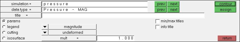
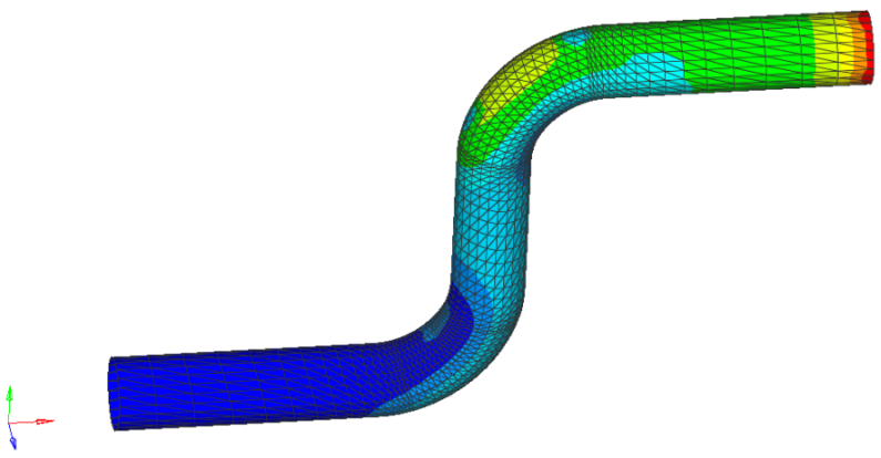
This simply displays the pressure load as a contour for an easier way to view the load. Now that the pressure load has been applied, an additional analysis can be set up and run.
|


