CFD-1800: Using Engineering Solutions, AcuSolve and HyperView to Perform a CFD Analysis

This tutorial uses:

•	Engineering Solutions (for meshing the CFD model)

•	AcuConsole (for setting up the model and submitting the job)

•	AcuSolve (for running the CFD simulation)

•	HyperView (for post-processing)

The model file used in this exercise can be found in the es.zip file. Copy the file(s) from this directory to your working directory.

Step 1: Launch Engineering Solutions and open the model file

1.	Click the Open Model icon on the Standard toolbar.

2.	Select the manifold_surf_mesh.hm file.

3.	Click Open to load the .hm file containing the surface mesh.

CFD-1800-01

Step 2: Load the CFD-AcuSolve user profile

1.	Click Preferences > User Profiles from the menu bar or click on the Standard toolbar.

2.	Click Engineering Solutions > CFD > AcuSolve.

Click OK.

Step 3: Check that all the elements in the collectors wall, inlet and outlet define a closed volume

1.	Click Mesh > Check > Component > Edges to open the Edges panel.

2.	Click comps and select the collectors wall, inlet and outlets.

3.	Click select, and then click find edges. A message indicating that no edges were found will appear on the status bar.

4.	Toggle free edges to T-connections.

5.	Select the three components again and then click find edges. The status bar will display "No T-connected edges were found."

6.	Click return to close the panel.

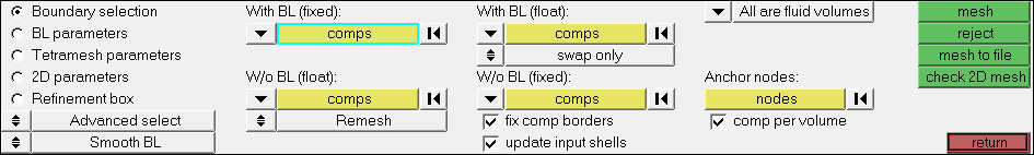
Step 4: Create the CFD mesh

1.	Click Mesh > Volume Mesh 3D > CFD tetramesh to open the CFD Tetramesh panel.

2.	Select the Boundary selection subpanel.

3.	Under the heading With BL (fixed), click comps and select the collector wall.

4.	Under the heading W/o BL (float), click comps and select the collectors inlet and outlets.

5.	Verify that the switch below the W/o BL (float) selector is set to Remesh. This means that the meshes in the zones defined by collectors inlet and outlets will be remeshed after being deformed by the boundary layer growth from adjacent surface areas.

6.	Select Smooth BL.

CFD-1800-03

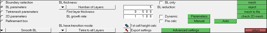
7. Click the BL parameters subpanel. All the data that has been entered in the Boundary selection subpanel is stored.

8. Select the options to specify the boundary layer and the tetrahedral core:

•	Number of Layers= 5

•	First layer thickness= 0.5

•	BL growth rate= 1.1

9. Under the BL hexa transition mode header, verify that the selection is set to Tetra to all Layers. This uses tetrahedral elements for the boundary layers.

10. Leave the BL only checkbox unchecked. This option generates the boundary layer alone and stops before generating the tetrahedral core.

CFD-1800-04

11. Click the Tetramesh parameters subpanel.

CFD-1800-05

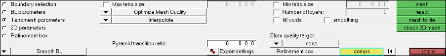
12. There are three different tetrameshing algorithms available. Select Optimize Mesh Quality.

13. Set the tetrahedral core growth rate, Interpolate. This avoids the problem of generating tetrahedral elements that are too large at the center of the core mesh.

14. Click mesh to create the CFD mesh. When this task is finished, two collectors are automatically created: CFD_bl001 and CFD_tetcore001.

15. Click return to close the panel.

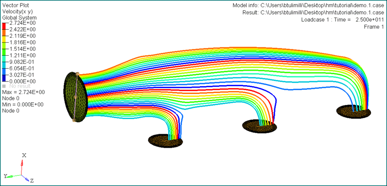
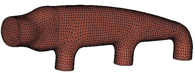
Step 5: Visualize and mask the generated mesh

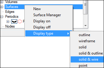
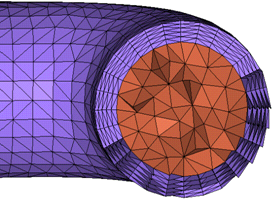
1.	To visualize the new mesh, set the element display to off for wall, inlet and outlets collectors.

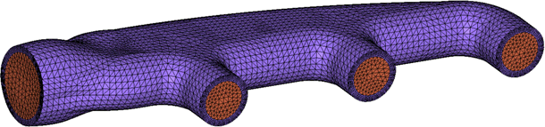
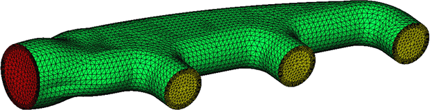
CFD-1800-06

2.	To mask the generated mesh use the shortcut key F5 and select the elements to be masked. The following is a snapshot. Observe the excellent mesh quality.

CFD-1800-07

Step 6: Organize the model

1.	Rename the collector CFD_Tetramesh_core as fluid. This collector will hold all the 3D volume elements.

2.	Click BCs>Organize to move all the elements from the collector CFD_boundary_layer to collector fluid.

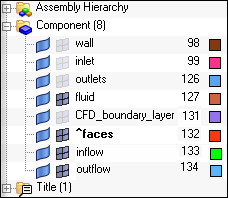
3.	Click BCs>Faces to automatically generate the collector ^faces containing all the external faces of the elements in collector fluid.

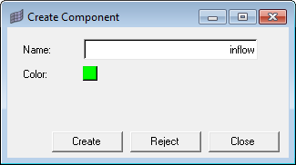
4.	Click BCs>Components>Single to create two new components named inflow and outflow.

CFD-1800-08

5.	In the Model browser, turn On the display ^faces component and put off the fluid component.

6.	Click BCs>Organize and click one element on the inlet/inflow plane (the element will become highlighted).

7.	Click elems>by face. All the elements in the collector ^faces on the inlet/inflow plane will be selected.

8.	Set the dest comp as inflow, and click move. Similarly, move the elements from ^faces associated with the outlets to the collector outflow.

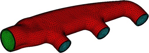
9.	Show the inflow and outflow components in the Model browser. When done, you will have all the exterior surfaces colored according to the collectors where they have been placed as shown in the image.

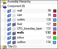
CFD-1800-09

CFD-1800-10

10.	The remaining elements in the collector ^faces are the walls. Rename collectors ^faces to walls.

Step 7: Exporting the model to AcuConsole

1.	Display only the components containing elements that have to be exported for AcuConsole. The components are: fluid, inflow, outflow, and walls. All other components should not be visible.

CFD-1800-11

2.	Click the icon in the CFD toolbar.

3.	In the File field, click the file icon and specify a name and location for the file.

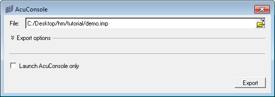
CFD-1800-13

3.	Click Export to launch AcuConsole and export a file.

The AcuConsole GUI opens with the model loaded.

CFD-1800-14

Step 1: Visualizing the model in AcuConsole

1.	Expand Surfaces and right-click Display Type to select solid & wire. This updates the model display with a mesh in the Visualization area.

CFD-1800-15

2.	For changing the color of a surface, right-click the surface and click Display Color. Select the desired color from the Select color dialog.

CFD-1800-16

Step 2: Set problem description and solution strategy

1.	Double-click Problem Description under Global.

CFD-1800-17

2.	In the panels area set the Title to Demo and Turbulence equation to Spalart-Allmaras.

CFD-1800-18

3.	Double-click Auto Solution Strategy and set the Relaxation factor to 0.4.

CFD-1800-19

Step 3: Set nodal initial condition and material model

1.	Double-click Nodal Initial Condition under Global.

2.	In the panels area set the X velocity to 2.0. Therefore, at the start of the simulation fluid is flowing with a velocity of 2 m/s.

CFD-1800-20

3.	In Model > Volumes > fluid tet4 > Element Set double-click Element Set and select Water in the drop down list next to Material model.

CFD-1800-21

Step 4: Set boundary conditions

1.	Right-click Surfaces and select Surface Manager. The Surface Manager dialog opens.

CFD-1800-22

2.	Make sure the Simple BC Active and Simple BC Type columns are present. If they are not shown clink Columns and select them.

3.	Under the Simple BC Type, make sure Inflow is set for fluid tet4 inflow tria3 surface, Outflow for fluid tet4 outflow tria3 and Wall for fluid tet4 walls tria3.

CFD-1800-23

4.	Click Close to close the dialog.

Step 5: Set inlet velocity

1.	Double-click Surfaces > fluid tet4 inflow tria3 > Simple Boundary Condition.

2.	In the panel area, select Inflow Type to Average velocity and Average velocity to 2.0 m/s.

CFD-1800-24

Step 6: Launch AcuSolve

1.	Click Tools > AcuSolve.

2.	Set the Problem name, Problem directory, Working directory, Number of processors, and so on, in this dialog.

3.	Click OK to launch AcuSolve.

When the job is submitted, AcuRun executes AcuPrep followed by AcuSolve.

AcuPrep reads the input file and prepares the data for AcuSolve to compute the solution.

The AcuTail window shows the status of the job.

CFD-1800-27

AcuProbe can be used for monitoring the job.

CFD-1800-28

Step 7: Launch AcuOut

AcuOut is a tool used to translate AcuSolve solution output to other formats. In this workshop the output has to be converted to EnSight format for loading to HyperView.

1.	Click Tools > AcuOut. The AcuOut GUI opens.

2.	Set the Output format to EnSight. Set the Data type, Variables, Time steps and format. Click Do next to Process.

CFD-1800-29

Step 1: Launch HyperView

HyperView can be launched several ways including:

•	Click Applications > HyperView from the menu bar.

•	On a Windows machine, click Start > Altair HyperWorks <version > HyperView.

•	On a LINUX machine, type hv in terminal window.

1.	Click the button next to Load model and Load results. Provide the location of case file generated using AcuOut.

CFD-1800-30

2.	Click Apply to load the model into HyperView.

Step 2: Boundary surface

The model is colored by geometry after loading.

1.	To color it by a scalar quantity, click the Contour icon on the Results toolbar.

2.	Select Pressure as the Result type and click Apply.

CFD-1800-31

Step 3: Cut plane

1.	Right-click within the Results browser and select Create > Section Cut. A section cut is automatically applied to the model, and the Section Cut panel is displayed.

2.	Verify that Define plane is set to Z Axis. Click Apply.

3.	Verify that Display Options has the Cross section option turned on. You can use the Define plane slider bar (located under the Z Axis button) to move the position of the section cut.

4.	Click the Contour icon on the Results toolbar.

5.	Select Velocity (v) as the Result type and click Apply.

CFD-1800-32

Step 4: Slice (or) clipping plane

1.	Within the Results browser expand the Section Cuts folder, right-click Section 1, and select Edit. The Section Cut panel opens.

2.	Under Display options select Clipping plane.

CFD-1800-34

Step 5: Velocity vectors

1.	In the Section Cut panel (under Display options) set it back to Cross section.

2.	Click the Vector panel icon on the Results toolbar.

3.	Under Selection (from the drop down list) select Sections.

4.	Click Sections to open the Extended Entity Selection. Select Displayed.

5.	Select X and Y components and click Apply.

CFD-1800-36

Step 6: Streamlines

1.	Within the Results browser, expand the Section Cuts folder. Click the icon before Section 1 to put off the display.

2.	Using the Results browser, turn off display for all components. Only turn On the display for SBC: fluid tet4 inflow tria3 and SBC: fluid tet4 outflow tria3 so that the inside of the flow domain is displayed in the graphics area.

3.	Click the Streamlines icon from the Results toolbar to open the Streamlines panel.

CFD-1800-38

4.	Click Add to add a new set of steamlines.

5.	Set the Rake type to Line.

6.	Click . This opens the Reference point dialog. Enter the Reference points as (X1: 66.96, Y1: 79.69, Z1: -400) and (X2: 28.9, Y2: 79.69, Z2: -400).

CFD-1800-40

7.	Enter 35 into the Number of seeds text box.

8.	Select Downstream from the Integration mode drop-down menu.

9.	Click Create Streamlines (located in the lower right hand corner of the panel.)

10.	Under Display options, change the Streamline size to 4 and hit Enter on the keyboard.

11.	Activate the Draw as tube option.

CFD-1800-39