In this tutorial, you will learn how to:

•	Create XY curves to define non-linear materials

•	Define beam elements with HyperBeam

•	Create constrained nodal rigid bodies

•	Create joints

•	Define *DEFORMABLE_TO_RIGID

•	Define *LOAD_BODY

•	Define *BOUNDARY_PRESCRIBED_MOTION_NODE

•	Use the HyperMesh Component Table tool to review the model’s data

Model Files

This tutorial uses the seat_start.hm and seat_2.hm files, which can be found in <hm.zip>/interfaces/lsdyna/. Copy the file(s) from this directory to your working directory.

Exercise 1: Define Model Data for the Seat Impact Analysis

This exercise will help you become familiar with defining LS-DYNA model data in HyperMesh.

In this exercise you will define and review model data for a LS-DYNA analysis of a vehicle seat impacting a rigid block. The seat and block model is shown in the image below.

HM-4610-05

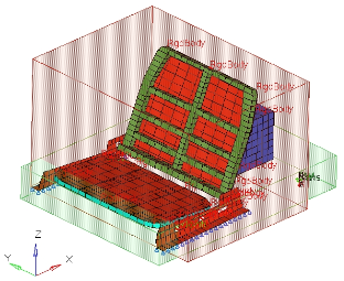
Seat and block model

Step 1: Load the LS-DYNA user profile

1.	Start HyperMesh Desktop.

2.	In the User Profile dialog, set the user profile to LsDyna.

Step 2: Retrieve the HyperMesh file

1.	Open a model file by clicking File > Open > Model from the menu bar, or clicking on the Standard toolbar.

2.	In the Open Model dialog, open the seat_start.hm file. The model appears in the graphics area.

3.	Observe the model using various visual options available in HyperMesh (rotation, zooming, etc.).

Step 3: Create an xy plot

1.	Open the Plots panel by clicking XYPlots > Create > Plots from the menu bar.

2.	In the plot= field, enter seat_mat.

3.	Set plot type to standard.

hm-4610-20

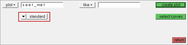
4.	Leave the like = field empty. When an existing plot is selected, the new plot adopts its attributes.

5.	Click create plot.

6.	Click return.

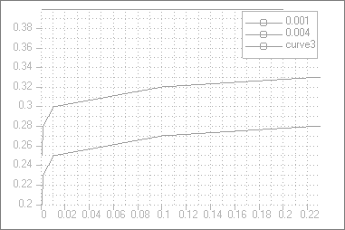
Step 4: Input data from a file to create two stress-strain curves

1.	Open the Read Curves panel by clicking XYPlots > Create > Curves > Read Curves from the menu bar.

2.	Leave the plot = field set to seat_mat.

3.	Click browse.

4.	In the Open dialog, open the file seat_mat_data.txt.

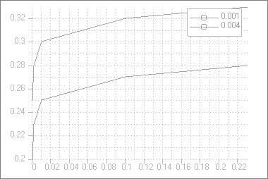
5.	Click input. HyperMesh creates two curves, and names them 0.001 and 0.004.

hm-4610-21

6.	Click return.

Step 5: Create a dummy xy curve to be used to create *DEFINE_TABLE

1.	Open the Edit Curves panel by clicking XYPlots > Edit > Curves from the menu bar.

2.	Go to the create subpanel.

3.	Click plot =, and select seat_mat.

4.	Select math.

5.	In the x = field, enter {0.0, 0.2}.

6.	In the y = field, enter {0.4, 0.4}.

hm-4610-35

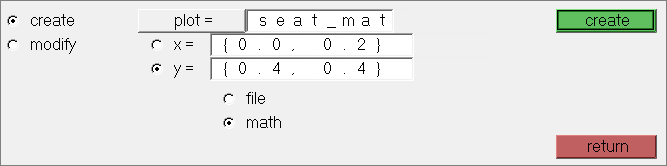
7.	Click create. HyperMesh creates a curve in the seat_mat plot, and names it curve3.

hm-4610-22

8.	Click return.

Step 6: Create *DEFINE_TABLE from the dummy curve

1.	In the Model browser, Curve folder, click curve3. The Entity Editor opens, and displays the curve's corresponding data.

hm-4610-7

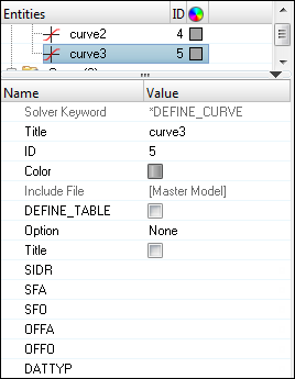
2.	Select the DEFINE_TABLE checkbox.

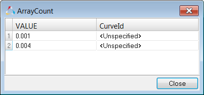
3.	For ArrayCount, enter 2.

Note:

This is the number of strain rate values to be specified.

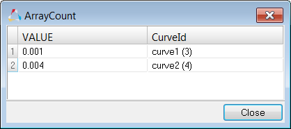
4.	In the Data: VALUE row, click .

5.	In the ArrayCount dialog, enter 0.001 in the strain rate VALUE(1) field and 0.004 in the strain rate VALUE(2) field.

hm-4610-8

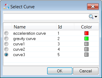
6.	In the CurveId(1) field, click Unspecified >> Curve.

hm-4610-10

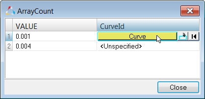
7.	In the Select Curve dialog, select curve1 and then click OK.

hm-4610-9

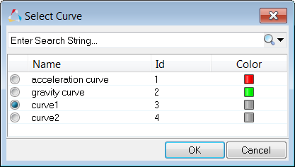
8.	In the CurveId(2) field, click Unspecified >> Curve.

9.	In the Select Curve dialog, select curve2 and then click OK.

10.	Click Close.

hm-4610-11

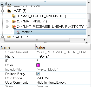
Step 7: Create the non-linear material (*MAT_PIECEWISE_LINEAR_PLASTICITY)

1.	Open the Solver browser by clicking View > Browsers > HyperMesh > Solver from the menu bar.

2.	In the Solver browser, right-click and select Create > MAT > MAT (1-50) > 24-MAT_PIECEWISE_LINEAR_PLASTICITY from the context menu. HyperMesh creates and opens a new material in the Entity Editor.

hm-4610-12

3.	For Name, enter steel.

4.	For Rho (Mass density), enter 7.8 E-6.

5.	For E (Young modulus), enter 200.

6.	For NU (Poisson ratio), enter 0.3.

7.	For SIGY (Yield stress), enter 0.25.

8.	Click LCSS, and then click curve.

hm-4610-13

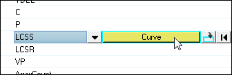
9.	In the Select Curve dialog, select curve3 and then click OK.

hm-4610-14

Step 8: Update the base_frame and back_frame components with the new non-linear material

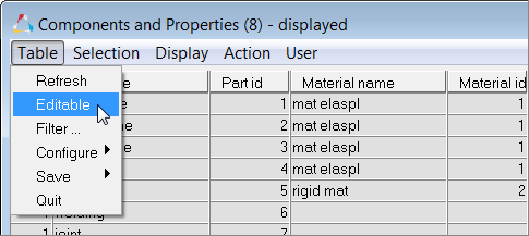
1.	From the menu bar, click Tools > Component Table.

2.	In the Components and Properties dialog, click Table > Editable from the menu bar.

hm-4610-36

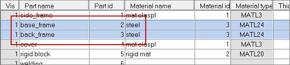
3.	Select the component, base_frame.

4.	Set Assign Values to Material name.

5.	Set HM-Mats to steel.

6.	Click Set. HyperMesh assigns the material steel to the component base_frame.

7.	In the Confirm dialog, click Yes.

8.	Assign the material steel to the component, back_frame.

hm-4610-23

9.	From the menu bar, click Table > Quit.

Steps 9-11: Create a beam element, *ELEMENT_BEAM, to complete the seat’s back_frame connection to the side_frame on the left side

Step 9: Restore a pre-defined view

1.	In the Model browser, View folder, right-click on Beam_view and select Show from the context menu.

Step 10: Set the current component to beams

1.	In the Model browser, Component folder, right-click on beams and select Make Current from the context menu. HyperMesh sets the beam component as the current collector.

Step 11: Create the beam

1.	Opens the Bars panel by clicking Mesh > Create > 1D Elements > Bars from the menu bar.

2.	Under orientation, click the switch and select node.

Note:

You will select a direction node later to define the beam’s section orientation.

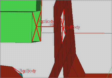
3.	Using the node A selector, select the center node of the left nodal rigid body.

4.	Using the node B selector, select the center node of the right nodal rigid body.

hm-4610-37

5.	Using the direction node selector, select any non-center node on one of the nodal rigid bodies. HyperMesh creates the beam.

hm-4610-38

6.	Click return.

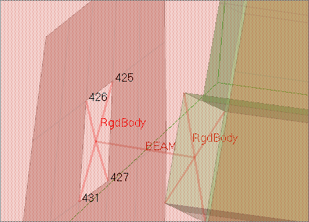
Step 12: Display node IDs for ease of following the next steps

1.	Open the Numbers panel by clicking on the Display toolbar.

2.	Set the entity selector to nodes.

3.	Click nodes >> by id.

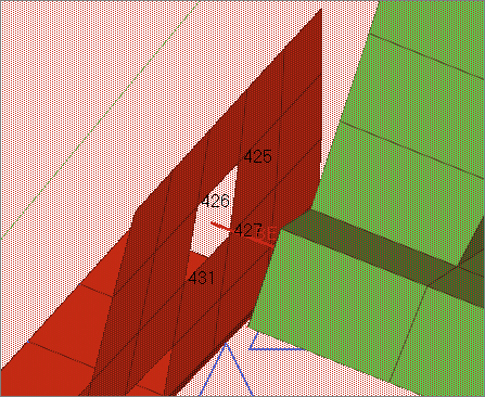
4.	In the id= field, enter 425-427, 431.

5.	Press ENTER.

6.	Select the display checkbox.

7.	Click on. HyperMesh displays the IDs.

hm-4610-39

8.	Click return.

Step 13: Set the current component to welding

1.	In the Model browser, Component folder, right-click on welding and select Make Current from the context menu. HyperMesh sets the welding component as the current collector.

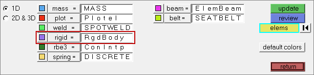
Step 14: Select the RgdBody type for the HyperMesh rigid configuration

1.	Open the Element Type panel by clicking Mesh > Assign > Element Type from the menu bar.

2.	Click rigid =, and then select RgdBody.

hm-4610-15

3.	Click update.

4.	Click return.

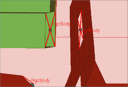
Step 15: Create the nodal rigid body (*CONSTRAINED_NODAL_RIGID_BODY)

1.	In the Solver browser, right-click and select Create > CONSTRAINED > CONSTRAINED_NODAL_RIGID_BODY > *CONSTRAINED_NODAL_RIGID_BODY from the context menu.

2.	In the Rigids panel, set the nodes 2-n selector to multiple nodes.

3.	Using the node1 selector, select the beam’s free end.

4.	Click nodes 2-n: nodes >> by id.

5.	In the id= field, enter 425, 426, 427, 431.

6.	Press ENTER.

hm-4610-40

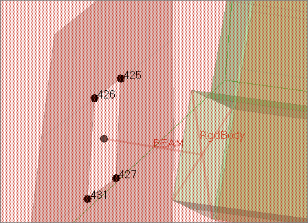
7.	Clear the attach nodes as set checkbox selected.

8.	Click create. HyperMesh creates the nodal rigid body.

hm-4610-41

9.	Click return. HyperMesh does not create *CONSTRAINED_JOINT_STIFFNESS; it is not needed for this joint to work.

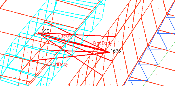
Step 16: Display node IDs for ease of following the next steps

1.	On the Visualization toolbar, click to display the model's elements as wireframe elements skin only.

2.	Opens the Numbers panel.

3.	Set the entity selector nodes.

4.	Click nodes >> by id.

5.	In the id= field, enter 1635, 1636.

6.	Press ENTER.

7.	Select the display checkbox.

8.	Click on. HyperMesh displays the IDs.

hm-4610-42

9.	Click return.

Step 17: Activate coincident picking

1.	Open the Graphics panel by clicking Preferences > Graphics from the menu bar.

2.	Select the coincident picking checkbox.

3.	Click return.

Step 18: Set the current component to joint

1.	In the Model browser, Component folder, right-click on joint and select Make Current from the context menu. HyperMesh sets the joint component as the current collector.

Step 19: Create a revolute joint between two nodal rigid bodies (*CONSTRAINED_JOINT_REVOLUTE)

Rigid bodies must share a common edge along which to define a joint. This edge, however, must not have nodes merged together. Two rigid bodies will rotate relative to each other along the axis defined by the common edge.

1.	In the Solver browser, right-click and select Create > CONSTRAINED > CONSTRAINED_JOINT_REVOLUTE > *CONSTRAINED_JOINT_REVOLUTE from the context menu.

2.	In the Joints panel, set joint type to revolute.

3.	Using the node 1 selector, click node 1635. The coincident picking mechanism displays two nodes: 1635 and 1633.

hm-4610-43

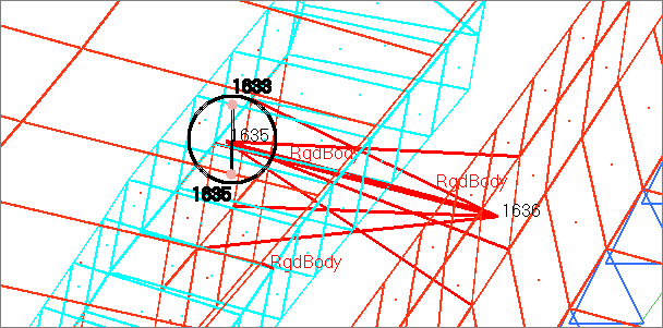
4.	From the coincident picking mechanism, click node 1635. Hypermesh selects node 1635 for node 1 in rigid body A.

5.	Using the node 2 selector, click node 1635. The coincident picking mechanism displays two nodes: 1635 and 1633.

6.	From the coincident picking mechanism, click node 1633. HyperMesh selects node 1633 for node 2 in rigid body B.

7.	Using the node 3 selector, click node 1636. The coincident picking mechanism displays two nodes: 1636 and 1634.

8.	From the coincident picking mechanism, click node 1636. HyperMesh selects node 1636 for node 3 in rigid body A.

9.	Using the node 4 selector, select node 1634 for node 4 in rigid body B.

10.	Click create. HyperMesh creates the joint.

11.	Click return.

Steps 20-22: Define *DEFORMABLE_TO_RIGID to set up the moving seat as rigid until the time of impact with the block, to reduce computation time

Step 20: Create an entity set that contains the components base_frame, back_frame, and cover

1.	In the Solver browser, right-click and select Create > SET > SET_PART > *SET_PART_LIST from the context menu. HyperMesh creates and opens a new set in the Entity Editor.

hm-4610-16

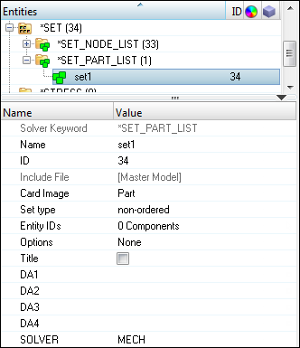
2.	For Name, enter set_part_seat.

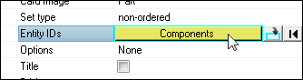
3.	For Entity IDs, click 0 Components >> Components.

hm-4610-17

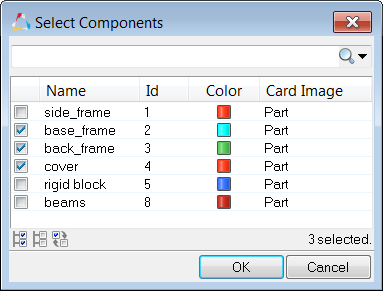
4.	In the Select Components dialog, select base_frame, back_frame, and cover and then click OK.

hm-4610-18

Step 21: Define *DEFORMABLE_TO_RIGID to switch the deformable seat to rigid at the beginning of the analysis

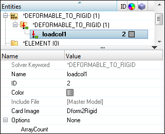
1.	In the Solver browser, right-click and select Create > DEFORMABLE_TO_RIGID > DEFORMABLE_TO_RIGID from the context menu. HyperMesh creates and opens a new load collector in the Entity Editor.

hm-4610-24

2.	For Name, enter dtor.

3.	For ArrayCount, select 1.

4.	For PSID, click Unspecified >> Set.

hm-4610-28

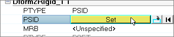
5.	In the Select Set dialog, select set_part_seat and then click OK.

6.	For MRB, click Unspecified >> Component.

7.	In the Select Component dialog, select rigid block and then click OK.

8.	Click Close.

Step 22: Create *DEFORMABLE_TO_RIGID_AUTOMATIC to switch the rigid seat to deformable when contact between the seat and block is detected

1.	In the Solver browser, right-click and select Create > DEFORMABLE_TO_RIGID > DEFORMABLE_TO_RIGID_AUTOMATIC from the context menu. HyperMesh creates and opens a new load collector in the Entity Editor.

hm-4610-25

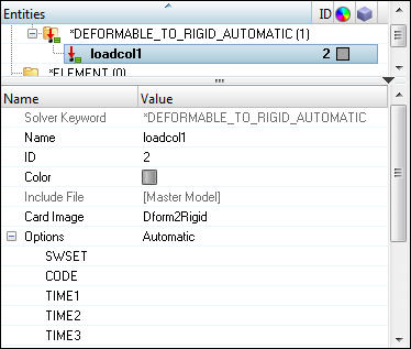
2.	For Name, enter dtor_automatic.

3.	For SWSET (set number of this automatic switch set), enter 1.

4.	Set CODE (activation switch code) to 0.

Note:

The switch will take place at [TIME1].

5.	For TIME1, enter 175.

Note:

The switch will not take place before this time.

6.	Select the R2D_Flag checkbox.

Note:

On export, the number of rigid parts to be switched to deformable is written to the R2D field (card 2, field 6). This number is based on the number of parts in the entity set you select next.

7.	Click PSIDR2D >> Set.

Note:

PSIDR2D is the part ID of the part which is switched to a rigid material.

hm-4610-26

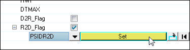
8.	In the Select Set dialog, select set_part_seat and then click OK.

Steps 23-27: Review the model’s component data using the Model Browser, Solver Browser or Component Table tool

Method 1: Using the Model browser

Step 23: Display only parts with a particular material (Ex: steel)

1.	In the Model browser, click .

hm-4610-44

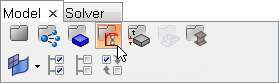
2.	In the ELASTIC-PLASTIC folder, MATL24 folder, right-click on steel and select Isolate from the context menu. HyperMesh only displays the components that have the selected material assigned.

3.	Review several materials, click , select a material, and scroll through the material using the arrow keys in the Model browser. The corresponding parts are automatically isolated in the view.

4.	Follow the above steps to select components using the By Properties option.

hm-4610-45

Step 24: Display all components

1.	In the Model browser, click .

Step 25: Rename a part

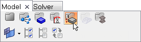
1.	In the Model browser, click .

2.	Right-click on the part you would like to rename, and then select rename from the context menu.

3.	In the editable field, enter a new name for the entity. The part's new name changes in the Solver and Model browsers.

Step 26: Renumber a part ID

1.	In the Model browser, click on a part's ID field. The ID field becomes editable.

2.	Enter a number that does not conflict with the existing part IDs, and then press Enter.

Method 2: Using the Solver browser

Step 23: Display only parts with a particular material (Ex: steel)

1.	In the Model browser, Materials folder, right-click on Steel and select Isolate from the context menu.

2.	In the Solver browser, *SECTION folder, select components based on properties.

Step 24: Display all components

1.	In the Solver browser, click the *MAT folder.

Step 25: Rename a part

1.	In the Solver browser, select the part you would like to rename. The Entity Editor opens, and displays the part's corresponding data.

2.	For Name, and enter a new name for the part. The part's new name changes in the Solver and Model browsers.

Step 26: Renumber a part ID

1.	In the Solver browser, select the part you would like to change the ID of. The Entity Editor opens, and displays the part's corresponding data.

2.	For ID, enter a new ID for the part. The part's new ID changes in the Solver and Model browser.

Method 3: Using the Component Table

Step 23: Display only parts with a particular material (Ex: steel)

1.	From the menu bar, click Tools > Component Table.

2.	In the Components and Properties dialog, click Display > By Material from the menu bar.

3.	In the panel area, click mats.

4.	Select the material, steel.

5.	Click Select.

6.	Click proceed. The Component Table only displays the components with the material steel assigned. All other components are turned off.

7.	To select components using the By Properties and By thickness options, repeat the above steps.

Step 24: Display all components

1.	From the menu bar, click Display > All. The table displays all of the components in the model.

Step 25: Rename a part

1.	From the menu bar, click Table > Editable. The table becomes editable. You can edit any of the columns that have a white background. For example, Part name, Part id, Thickness, and so on.

2.	Click any Part name field. The field becomes editable.

3.	Enter a new name for the part.

4.	In the Confirm dialog, click Yes. The part's new name changes in the Solver and Model browsers.

Step 26: Renumber a part ID

1.	From the menu bar, click Table > Editable. The table becomes editable.

2.	Click any Part Id field. The field becomes editable.

3.	Enter a new ID that does not conflict with any existing part IDs.

4.	In the Confirm dialog, click Yes. The part's new ID changes in the Solver and Model browsers.

Step 27: Review the model’s data using the Solver Browser

The created solver entities are listed in the Solver browser, within their corresponding folders. Use the following options on each entity to help navigate through the model: Show, Hide, Isolate, and Review.

1.	In the Solver browser, *DEFORMABLE_TO_RIGID folder, right-click on dtor and select Isolate Only from the context menu. HyperMesh only displays the entities that are referred in this keyword.

2.	Highlight the entities that are referenced by this keyword by right-clicking on dtor and selecting Review from the context menu.

3.	Right-click on the folder *BOUNDARY and then select Show from the context menu. HyperMesh displays the entities on which the loads in the folder are defined, as well as the load handles.

Exercise 2: Define Boundary Conditions and Loads for the Seat Impact Analysis

This exercise will help you become familiar with defining LS-DYNA boundary conditions and loads using HyperMesh.

In this exercise, you will define boundary conditions and load data for an LS-DYNA analysis of a vehicle seat impacting a rigid block. The seat and block model is shown in the image below.

HM-4610-05

Seat and block model

This exercise contains the following three tasks.

•	Define gravity acting in the negative z-direction with *LOAD_BODY_Z

•	Define the seat’s acceleration with *BOUNDARY_PRESCRIBED_MOTION_NODE

•	Export the model to an LS-DYNA 970 formatted input file and submit it to LS-DYNA

Step 1: Make sure the LS-DYNA user profile is still loaded

1.	Start HyperMesh Desktop.

2.	In the User Profile dialog, set the user profile to LsDyna.

Step 2: Retrieve the HyperMesh file

1.	To open a model file, click File > Open > Model from the menu bar, or click on the Standard toolbar.

2.	In the Open Model dialog, open the seat_2.hm file. The model appears in the graphics area.

3.	Observe the model using various visual options available in HyperMesh (rotation, zooming, etc.).

Step 3: Define gravity acting in the negative z-direction with *LOAD_BODY_Z

1.	In the Solver browser, right-click and select Create > LOAD > LOAD_BODY_Z from the context menu. HyperMesh creates and opens a new load collector in the Entity Editor.

hm-4610-31

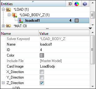
2.	For Name, enter gravity.

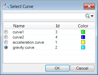
3.	Click LCID, and then click curve.

hm-4610-32

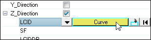
4.	In the Select Curve dialog, select gravity curve and then click OK.

hm-4610-33

5.	For SF (scale factor for acceleration in z-direction), enter 0.001.

Steps 4-6: Define the seat’s acceleration with *BOUNDARY_PRESCRIBED_MOTION_NODE

Step 4: Create a load collector for the acceleration loads to be created

1.	In the Model browser, right-click and select Create > Load Collector from the context menu. HyperMesh creates and opens a new load collector in the Entity Editor.

hm-4610-34

2.	For Name, enter accel.

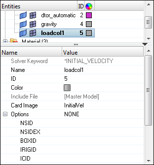
3.	Set Card Image to <None>.

4.	Optional. Click the Color icon, and select a color for the load collector.

Step 5: Create acceleration loads on nodes

1.	Open the Accelerations panel by clicking BCs > Create > Accelerations from the menu bar.

2.	Click load types =, and select PrcrbAcc_S.

3.	Click sets.

4.	Select the set, accel_nodes.

5.	Click select.

6.	Click the magnitude= switch, and select curve, vector.

7.	In the magnitude= field, enter 0.001.

Note:

This is the scale factor for the pre-defined curve to be specified in the next step for the acceleration loads. It will define the seat’s acceleration as a function of time.

8.	Set the orientation selector to x-axis.

Note:

This is the x-translational degree of freedom.

9.	Double-click curve.

10.	Select the curve, acceleration curve.

11.	In the magnitude% = field, enter 1.0E+7.

Note:

This is the scale factor for the graphical representation of the acceleration loads. It does not affect the actual acceleration value.

12.	Click create. HyperMesh creates the acceleration loads.

13.	Click return.

Step 6: Export the model to an LS-DYNA 971 formatted input file

1.	From the menu bar, click File > Export > Solver Deck.

2.	In the Export - Solver Deck tab, set File type to Ls-Dyna.

3.	In the File field, navigate to your working directory and save the file as seat_complete.key.

4.	Click Export.

Step 7 (Optional): Submit the LS-DYNA input file to LS-DYNA 971

1.	From the Start menu on your desktop, open the LS-DYNA Manager program.

2.	From the solvers menu, select Start LS-DYNA analysis.

3.	Load the file seat_complete.key.

4.	Click OK to start the analysis.

Step 8 (Optional): View the results in HyperView

The exercise is complete. Save your work as a HyperMesh file.

HM-4610: Using Curves, Beams, Rigid Bodies, Joints, and Loads in LS-DYNA

HM-4610: Using Curves, Beams, Rigid Bodies, Joints, and Loads in LS-DYNA

HM-4610: Using Curves, Beams, Rigid Bodies, Joints, and Loads in LS-DYNA

Model Files

Exercise 1: Define Model Data for the Seat Impact Analysis

Steps 9-11: Create a beam element, *ELEMENT_BEAM, to complete the seat’s back_frame connection to the side_frame on the left side

Steps 20-22: Define *DEFORMABLE_TO_RIGID to set up the moving seat as rigid until the time of impact with the block, to reduce computation time

Steps 23-27: Review the model’s component data using the Model Browser, Solver Browser or Component Table tool

Method 1: Using the Model browser

Method 2: Using the Solver browser

Method 3: Using the Component Table

Exercise 2: Define Boundary Conditions and Loads for the Seat Impact Analysis

See Also: