HS-1505: Register a Templex Function in HyperStudy

In this tutorial you will learn how to register a Templex function in HyperStudy. The objective of this tutorial is to find the RADIOSS material parameter values so that the stress-strain curve of the tensile test simulation matche the tensile test experimental curve.

By the end of this tutorial, you will know how to:

•	Create an input template from a RADIOSS file using the HyperStudy - Editor

•	Setup a study

•	Run a system identification optimization study

The sample base input template used in this tutorial can be found in <hst.zip>/HS-1505/. Copy the files TENSILE_TEST_0000.rad, TENSILE_TEST_0001.rad, experiment.xy, and area_bw_two_curves.mvw from this directory to your working directory. The mvw file has a function that calculates the area between two curves.

A quarter of a standard tensile test specimen is modeled using symmetry conditions. A traction is applied to a specimen via an imposed velocity at the left-end.

The units are: mm, ms, g, N, MPa.

hs_1505_1

Geometry of the Tensile Specimen (One Quarter of the Specimen is Modeled)

hs_1505_2

Sections of Node Saved for Time History

The material to be characterized is a 6063 T7 Aluminum. It has an isotropic elasto-plastic behavior which can be reproduced by a Johnson-Cook model without damage (RADIOSS Block Law2), defined as follows:

hs_1505_function

hs_1505_intro

In this tutorial, the parameters a, b, n, σmax (maximum stress), and the Young modulus are defined as input variables. The stress-strain curve obtained by the experimental test is shown in the following image.

hs_1505_3

Engineering Stress Versus Engineering Strain Curve (Experimental Data)

For the simulation results, engineering strains will be obtained by dividing the displacement of node 1 by the reference length (75 mm), and engineering stresses will be obtained by dividing the force in section 1 by its initial surface (12.012 mm2).

hs_1505_4

Engineering Stress Versus Strain Curve (Simulation Results)

In this step, you can create the base input template in HyperStudy or use the base input template in the study Directory.

1.	Start HyperStudy.

2.	From the menu bar, click Tools > Editor. The Editor opens.

3.	In the File field, open the TENSILE_TEST_0000.rad file.

4.	In the Find area, enter /MAT/PLAS_JOHNS/1.

5.	Click . HyperStudy highlights /MAT/PLAS_JOHNS/1.

hs_1505_find word

6.	Select variable E by highlighting the first 20 fields in row 51.

Tip:	Quickly highlight 20-character fields by pressing CTRL to activate the Selector (set to 20 characters) and then clicking the value.

hs_1505_e_field

7.	Right-click on the highlighted fields and select Create Parameter from the context menu.

8.	In the Parameter-varname_1 dialog, Label field, enter E_Young.

9.	Set the Lower Bound to 50000, the Initial Bound to 60400, and the Upper Bound to 70000.

10.	In the Format field, enter %20.5f.

hs_1505_design variable properties

11.

Click OK.

12.	Define four more variables using the information provided in the table below.

Variable	Label	Lower Bound	Initial Value	Upper Bound	Format
a	a_PlasticityYieldStress	90	110	120	%20.5f
b	b_HardeningCoeff	100	125	160	%20.5f
n	n_HardeningExpo	0.1	0.2	0.3	%20.5f
sigmax	Sigma_Max	250	280	290	%20.5f

13.	Click Save.

14.	In the Save Template dialog, save the file as TENSILE_TEST_0000.tpl.

15.	Close the Editor.

1.	From the menu bar, click File > Use Preferences File.

2.	In the HyperStudy - Set Preference File dialog, open the area_bw_two_curves.mvw file.

1.	To start a new study, click File > New from the menu bar, or click on the toolbar.

2.	In the HyperStudy – Add dialog, enter a study name, select a location for the study, and click OK.

3.	Go to the Define Models step.

4.	Add a Parameterized File model.

a.	From the Directory, drag-and-drop the TENSILE_TEST_0000.tpl file into the work area.

hs_1505_drag_drop_model

b.	In the Solver input file column, enter TENSILE_TEST_0000.rad ; TENSILE_TEST_0001.rad. This is the name of the solver input file HyperStudy writes during any evaluation.

c.	In the Solver execution script column, select RADIOSS (radioss).

d.	In the Solver input arguments column, enter -both at the end of $file. This solver input argument runs the Starter and the Engine of RADIOSS for the crash analysis, and also prevents the creation of the .h3d result file from animation files.

Note:

X is the number of CPUs to use for the simulation.

5.	Click Import Variables. Five input variables are imported from the TENSILE_TEST_0000.tpl resource file.

6.	Go to the Define Input Variables step.

7.	Review the input variable's lower and upper bound ranges.

8.	Go to the Specifications step.

1.	In the work area, set the Mode to Nominal Run.

2.	Click Apply.

3.	Go to the Evaluate step.

4.	Click Evaluate Tasks. An approaches/nom_1/ directory is created inside the study directory. The approaches/nom_1/run__00001/m_1 directory contains the TENSILE_TESTT01 file, which consist of the time history results of the simulation.

5.	Go to the Define Output Responses step.

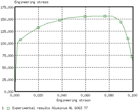
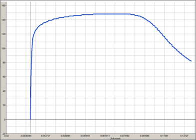
In order to fit the RADIOSS stress-strain curve to the experimental data, you need to compare the two curves. In this step, you will use the external temple function area_bw_two curves. (Tutorial 4200: Uses system identification to solve the same problem.)

1.	Create an output response labeled Area Between Two Curves.

a.	Click Add Output Response.

b.	In the HyperStudy - Add dialog, add one output response and label it Area Between Two Curves.

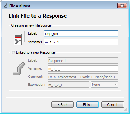
2.	Create a file source labeled Disp_sim.

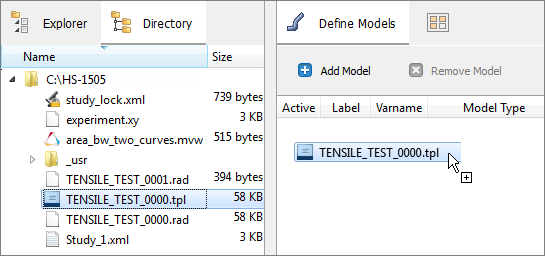
a.	From the Directory, drag-and-drop the TENSILE_TEST01 file, located in approaches/nom_1/run_00001/m_1, into the work area.

b.	In the File Assistant dialog, set the Reading technology to Altair® HyperWorks® and click Next.

c.	Select Single item in a time series, then click Next.

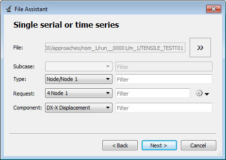
d.	Define the following options, then click Next.

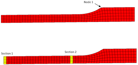
•	Set Type to None/Node 1.

•	Set Request to 4 Node 1.

•	Set Component to DX-X Displacement.

hs_1505_disp_sim

e.	Label the File Source Disp_sim.

f.	Clear the Linked to a new Response checkbox.

g.	Click Finish

hs-4200-1

3.	Create a second file source labeled Force_sim by repeating step 1, except select the following options:

•	Set Type to Section/SECTION_2.

•	Set Request to 2 section 1.

•	Set Component to FT-Resultant Tangent Force.

4.	Create a third file source labeled Strain_exp.

a.	In the Expression column of the output response Area Between Two Curves, click .

b.	In the Expression Builder, File Sources tab, click Add File Source.

c.	In the Add - HyperStudy dialog, define the file source and click OK.

•	Label the file source Strain_exp.

•	Select the type Reference file.

d.	In the File column of the file source, click .

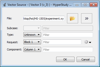
e.	In the Vector Source dialog, define the vector and click OK.

•	In the File field, navigate to your working directory and open the experiment.xy file.

•	Set Type to Unknown.

•	Set Request to Block1.

•	Set Component to Column 1.

hs_1505_vector_3

5.	Create a fourth file source labeled Stress_Exp by repeating step 4, except select the following options:

•	Set Type to Unknown.

•	Set Request to Block1.

•	Set Component to Column 2.

6.	Define the Area Between Two Curves output response.

a.	In the Expression Builder, click the Functions tab.

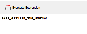
b.	From the list of available functions, select area_between_two_curves.

c.	Click Insert Varname. The function area_between_two_curves(,,,) appears in the Evaluate Expression field.

hs_1505_insert varname

d.	In a text editor, open the area_bw_two_curves.mvw file. The text editor displays the following:

function area_between_two_curves(v1x,v2x,v1y,v2y)

{

newx = sync2(v1x, v2x)

newy1 = lininterp(v1x, v1y, newx)

newy2 = lininterp(v2x, v2y, newx)

suby = newy1-newy2

area_value = absarea(newx, suby)

return area_value

}

With arguments x_sim, x_test, y_sim, y_test.

e.	In the Expression Builder, Evaluate Expression field, edit the expression so that it reads area_between_two_curves(m_1_v_1,v_3,m_1_v_2,v_4).

Note:

You are reading displacements and forces from the simulation, whereas from the experiment you have strains and stresses. Convert the displacement and forces to strains and stresses by dividing the displacements by the length (75) and forces by the area (12).

f.	Edit the function again, so that it reads area_between_two_curves(m_1_v_1/75,v_3,m_1_v_2/12,v_4)

g.	Click Evaluate Expression.

Click OK.

1.	In the Explorer, right-click and select Add Approach from the context menu.

2.	In the HyperStudy - Add dialog, select Optimization and click OK.

3.	Go to the Select Input Variables step.

4.	Review the input variable's lower and upper bound ranges.

5.	Go to the Select Output Responses step.

6.	Add an objective.

a.	Click the Objectives tab.

b.	Click Add Objective.

c.	In the HyperStudy - Add dialog, add one objective.

d.	Define the objective.

•	Set Type to Minimize.

•	Set Apply On to Area Between Two Curves (r_1).

7.	Click Apply.

8.	Go to the Specifications step.

9.	In the work area, set the Mode to Adaptive Response Surface Method (ARSM).

Note:

Only the methods that are valid for the problem formulation are enabled.

10.	Click Apply.

11.	Go to the Evaluate step.

12.	Click Evaluate Tasks.

13.	Optional. Click the Evaluation Plot tab to plot the optimization iteration history for the objective.

hs_1505_plot 2d

14.	Optional. Click the Iteration History tab to review the iteration history in a table.

HS-1505: Register a Templex Function in HyperStudy

HS-1505: Register a Templex Function in HyperStudy

HS-1505: Register a Templex Function in HyperStudy

Variable

Label

Lower Bound

Initial Value

Upper Bound

Format

See Also: