HS-1620: Settings Up a Flux Model

An electromagnetic actuator is a device that converts an electric current into a mechanical output. In this tutorial, you will be investigating the relationship between actuator dimensions and the mechanical force output. The actuator is composed of an U magnetic core, mobile magnetic part, and two coils supplied by an amp-turn number. The finite element model is created and analyzed by Flux. The Flux model also contains the input variables and output responses of interest.

hs_1620_electromagnetic_actuator_and_finite_element_model

Electromagnetic actuator and its Finite element model

hs_1620_design_variables_2

Input variables

The files used in this tutorial can be found in <hst.zip>/HS-1620/. Copy the tutorial files from this directory to your working directory.

Note:

This tutorial requires registration of the installed version of Flux Software with HyperStudy. For details, see Flux Model.

1.	Start HyperStudy.

2.	To start a new study, click File > New from the menu bar, or click on the toolbar.

3.	In the HyperStudy – Add dialog, enter a study name, select a location for the study, and click OK.

4.	Go to the Define models step.

5.	Add a Flux model by dragging-and-dropping the Example.F2G from the Directory into the work area.

hs_1620_add_model_flux

The Resource, Solver input file, Solver execution script, and Solver input arguments fields become populated.

hs_1620_define_model

6.	Click Import Variables. Ten input variables are imported from the Example.F2G file.

7.	Go to the Define Input Variables step, and review the input variables.

hs_1620_design_variables

8.	Go to the Specifications step.

1.	In the work area, set the Mode to Nominal Run.

2.	Click Apply.

3.	Go to the Evaluate step.

4.	Click Evaluate Tasks. An approaches/nom_1/ directory is created inside the study directory. The approaches/nom_1/run__00001/m_1 sub-directory contains the run files.

5.	Go to the Define Output Responses step.

1.	Review the output responses.

hs_1620_define_responses

2.	Click Evaluate Expressions to extract output response values.

3.	Click OK. This complete the study setup.

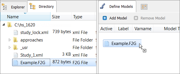
1.	In the Explorer, right-click and select Add Approach from the context menu.

2.	In the HyperStudy - Add dialog, add a Stochastic.

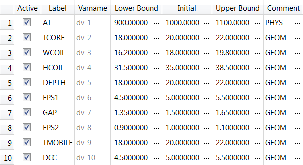
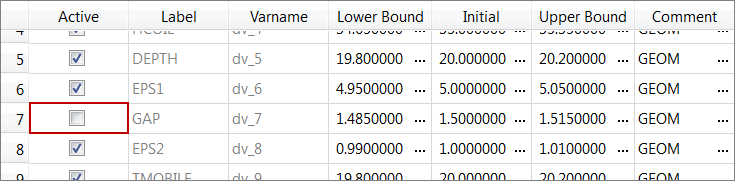
3.	In the Select Input Variables step, clear the Active checkbox for GAP.

hs_1620_select_dvs_stoachastic

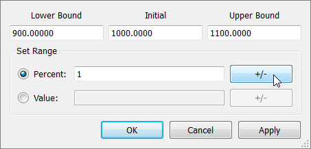
4.	For each input variable, adjust the lower and upper bounds, which will be used to calculate statistical distribution settings, in this case the variance of normal distribution.

a.	In the Initial column, click .

b.	In the window, enter 1 in the percent field and click +/-.

Click OK.

hs_1620_change_dv_bounds

5.	Go to the Specifications step.

6.	In the work area, set the Mode to Hammersley.

7.	In the Settings tab, verify that the Number of runs is 100.

Note:

If you are using a laptop with a Win64 operating system, 32 GB ram, Intel Core i7 CPU, it may take around 40 minutes to run 100 Flux simulations. To reduce the run times, change the Number of Runs to a lower value. However, a high number of runs is necessary for better statistical accuracy.

8.	Click Apply.

9.	Go to the Evaluate step.

10.	Click Evaluate Tasks.

11.	Go to the Post processing step.

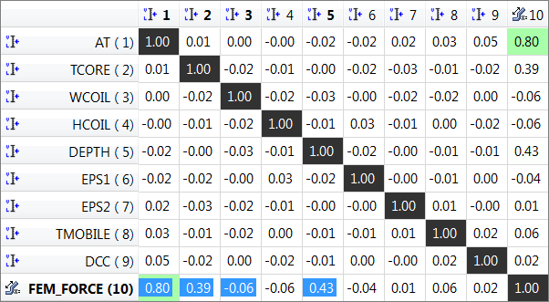
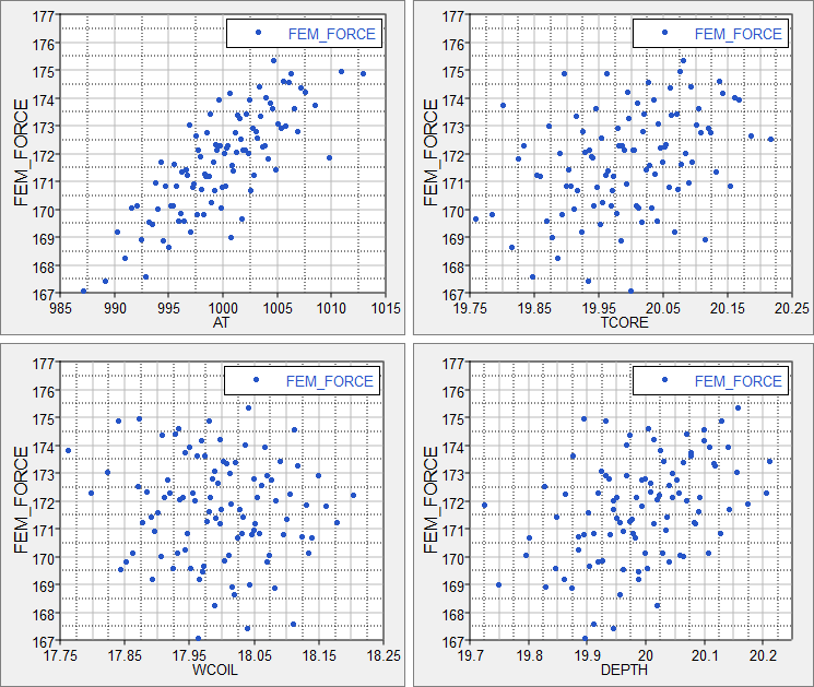
12.	Click the Scatter 2D tab to plot correlation values.

Correlation measures the strength and direction between associated variables. Correlation coefficients can have a value from -1 to 1; -1 indicates a strong but negative correlation and 1 indicates a strong and positive correlation.

The correlation values for variables AT, DEPTH, and TCORE with Force are 0.80, 0.43, and 0.39, which indicates that Force is correlated to AT and Force is somewhat correlated to DEPTH and TCORE. These three correlations are positive, meaning that you should expect to see an increase in Force corresponding to an increases in AT, DEPTH, and TCORE. You can also expect to see no changes in Force corresponding to changes in other variables. DEPTH and TCORE are somewhat correlated to FORCE, therefore you may see deviations from these predicted behaviors.

hs_1620_correlation

You can visualize these correlations in the Scatter2D plot. In the plot for FORCE vs AT, you can see the design cloud follows a nice pattern of increasing Force with increasing AT. In the plot for WCOIL vs FORCE, you should not observe any relationship between the two.

hs_1620_scatter2d