HS-1810: Post Proceesing with HyperStudy

This tutorial demonstrates how to post process studies with HyperStudy. We will use the model described in the HyperStudy tutorial HS-4415 and create various appraoches (Design of Experiment, Approximation, Optimization, Stochastic) to illustrate the rich variety of tools and post processing methods offered by HyperStudy.

Before running this tutorial, you must complete tutorial HS-4415: Optimization Study of a Landing Beam using Excel or you can import the archive file HS-4415.hstx, available in <hst.zip>/HS-1810/.

1.	In the Explorer, right-click and select Add Approach from the context menu.

2.	In the HyperStudy - Add dialog, select Doe and click OK.

3.	Go to the Select Input Variables step.

4.	Review the input variable's lower and upper bound ranges.

5.	Go to the Specifications step.

6.	In the work area, set the Mode to Fractional Factorial.

7.	Click Apply.

8.	Go to the Evaluate step.

9.	Click Evaluate Tasks.

10.	While the DOE is in progress, click the Tasks tab to view the feedback on the results of the evaluation.

11.	During the execution of the DOE, you can monitor the evaluation of the 16 runs in either the Evolution Plot or Evolution Data tabs.

12.	Go to the Post processing step.

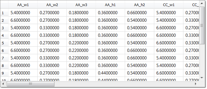
1.	Click the Summary tab to view all input variable and output response run data in a table.

Tip: Use the Sort and Find options in the right-click context menu to sort and search data.

hs_1810_run_summary

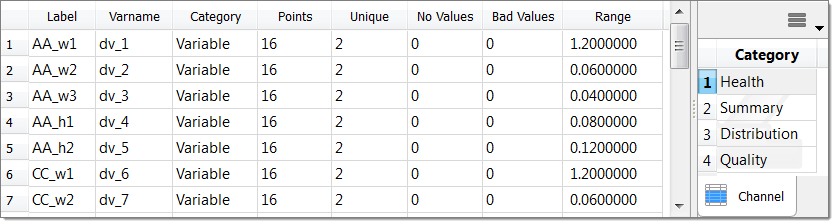
2.	Click the Integrity tab to view statistical measures over the population (samples of the DOE) for all of the input variables and output responses.

hs_1810_stats

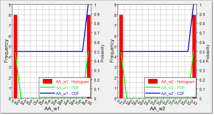
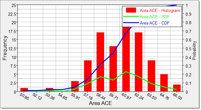
3.	Click the Distribution tab to view a histogram of the Doe results.

Display the entities in one or multiple plots by clicking . Each plot presents the range of the entity in abscissa (an input variable or an output response), the histogram (red bar chart for frequency), probability distribution function (PDF in green) and cumulative probability distribution function (CDF in blue).

hs_1810_histogram

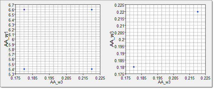
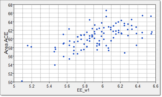
4.	Click the Scatter 2D tab to plot the Doe results.

Use the Channel selector to select entities to plot. Select one entity for the X-Axis, and select one or more entities for the Y-Axis.

hs_1810_scatter_2d

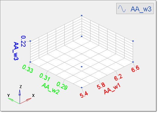
5.	Click the Scatter 3D tab to view Doe results in a scatter plot.

Only one input variable/output response can be selected for the X and Y axes, whereas multiple input variables/output responses can be selected for the Z axis.

1800scat3

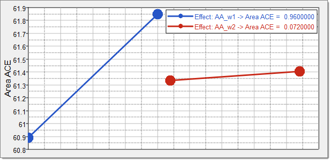
6.	Click the Linear Effects tab to plot the effect of an input variable on an output response, ignoring the effects of other input variables.

7.	Using the Channel selector, select the variables AA_w1 and AA_w2 and the output response Area ACE.

1800_main_effects

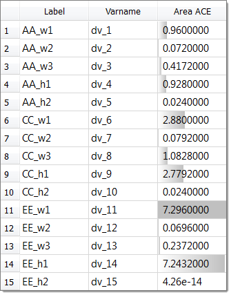
8.	Click the Effects Table tab to displays the effects of input variables on the output responses, ignoring the effects of other input variables.

Tip: From the Channel selector, use the Sort and Filter options in the right-click context menu to sort and filter effects.

1800_effects_table

1.	Repeat Step 1: Run a DOE Study to add a second DOE to the study. In the Specifications step, set the Mode to Hammersley and change the Number of runs to 50.

2.	Repeat Step 1: Run a DOE Study once more to add a third DOE to the study. In the Specifications step, set the Mode to Latin HyperCube and change the Number of runs to 15.

1.	In the Explorer, right-click and select Add Approach from the context menu.

2.	In the HyperStudy - Add dialog, select Fit and click OK.

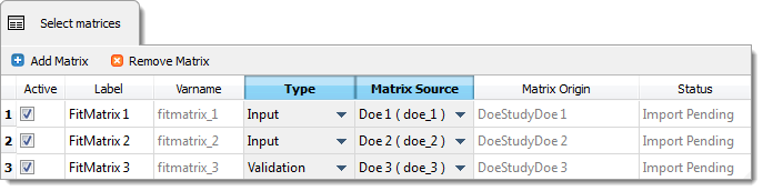
3.	Go to the Select matrices step.

4.	Click Add Matrix.

5.	In the HyperStudy - Add dialog, add three matrices.

6.	Define FitMatrix1, FitMatrix2, and FitMatrix3 by selecting the options indicated in the image below from the Type and Matrix Source columns.

hs_1810_select_matrices

7.	Click Import Matrix.

8.	Go to the Specifications step.

9.	In the work area, set the Mode to Radial Basis Function (RBF).

10.	Click Apply.

11.	Go to the Evaluate step.

12.	Click Evaluate Tasks.

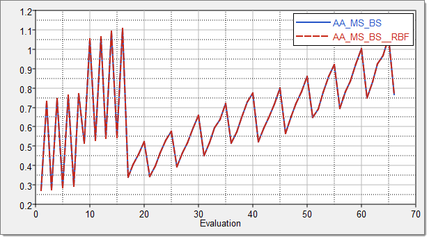
13.	To review the values of the output responses and their approximations while the evaluation is in progress, click the Evaluation Data and Evaluation Plot tabs.

hs_1810_evolution_plot

14.	Go to the Post processing step.

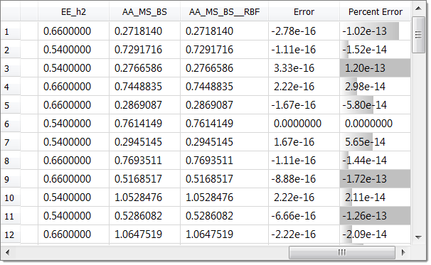
1.	Click the Residuals tab to identify errors for each design.

The error (and percentage) between the original output response and the approximation is listed for each run of the input, cross-validation, or validation matrices.

1800fit_residuals

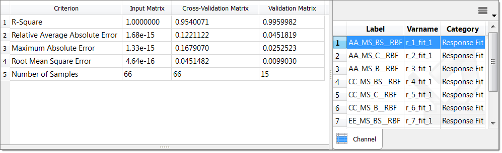
2.	Click the Diagnostics tab to assess the accuracy of a Fit. Different criteria is displayed for the Input, Validation, and merged matrices.

Use the Channel selector to select a specific output response for which to review diagnostics.

1800_fit_diag

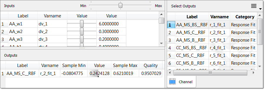
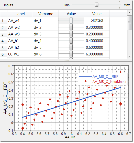
3.	Click the Trade-Off 1D tab to modify the values of input variables in order to see their effect on the output response approximations.

Use the Channel selector to select the desired output responses to display. Input variable controls are located in the in the top frame (Inputs). Change each input variable by moving the slider in the first Value column, or by entering a value into the second Value column. Set input variables to their initial, minimum, or maximum values by moving the slider in the upper right-hand corner of the Inputs frame.

1800_tradeoffs

4.	Click the Trade-Off 2D and Trade-Off 3D tabs to plot variables and output responses in order to see the input variables effect on the output response approximations.

In both of these tabs, use the Channel selector to select input variables and output responses to plot. The values for the input variables which are not plotted are modified in the top frame (Inputs). Move the sliders in the Value column to modify the other input variables, while studying the output response throughout the design space.

1800_scatters_tab

1.	In the Explorer, right-click and select Add Approach from the context menu.

2.	In the HyperStudy - Add dialog, select Optimization and click OK.

3.	Repeat the same optimization setup as in tutorial HS-4415-Step 4: Add an Optimization Approach and a Run Optimization. Just as Optimization 1, Optimization 2 should have one objective function and nine constraints.

1.	Go to the Select Input Variables step.

2.	Review the input variable's lower and upper bound ranges.

3.	Go to the Select Output Responses step.

4.	Click Add Objective.

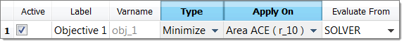
5.	In the HyperStudy - Add dialog, add one objective.

6.	Define the objective.

a.	Set Type to Minimize.

b.	Set Apply On to Area ACE (r_10).

hs_1810_objective1

7.	Click the Constraint tab.

8.	Click Add Constraint.

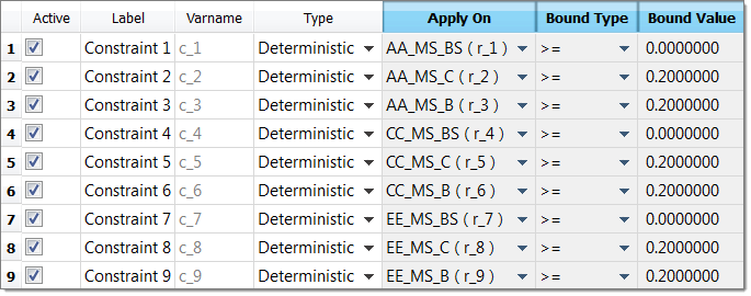
9.	In the HyperStudy - Add dialog, add nine constraints.

10.	Define Constraint 1 through Constraint 9 by selecting the options indicated in the image below from the Apply On, Bound Type, and Bound Value columns.

hs_4415_constraints

11.	Click Apply.

4.	Go to the Specifications step.

5.	In the work area, set the Mode to Adaptive Response Surface Method (ARSM).

Note:

Only the methods that are valid for the problem formulation are enabled.

6.	Click Apply.

7.	Go to the Evaluate step.

8.	Click Evaluate Tasks to launch the Optimization.

9.	Click the Evaluation Plot tab to plot variables and output responses across runs (abscissa are run numbers, not iterations).

1800_evplot

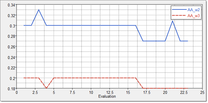
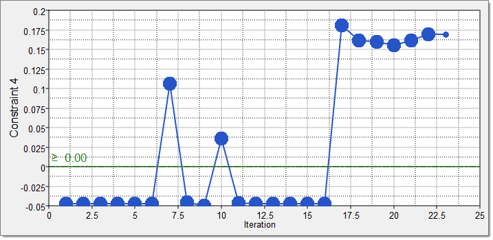
10.	Click the Iteration Plot tab to plot variables and output responses against iterations.

1800multiobj

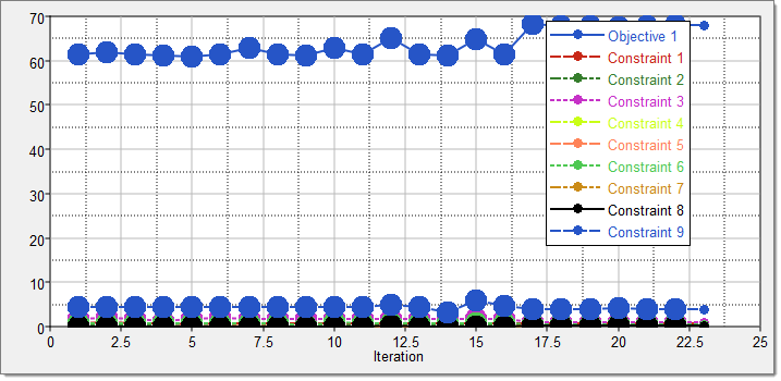
When the constraint history is plotted, the constraint bounds can be marked with a datum line. Use the Channel selector to select a constraint, then click (located above the Channel selector) and select Bounds.

hs_1810_bounds

1.	In the Explorer, right-click and select Add Approach from the context menu.

2.	In the HyperStudy - Add dialog, select Stochastic and click OK.

3.	Go to the Specifications step.

4.	In the work area, set the Mode to Hammersley.

5.	In the Settings tab, change the Number of runs to 100.

6.	Click Apply.

7.	Go to the Evaluate step

8.	Click Evaluate Tasks.

9.	Go to the Post processing step.

During the Post Processing step of a Stochastic approach, you can access additional result analysis tools.

1.	Click the Integrity tab to access a series of statistical measures on input variables and output responses.

2.	Click the Distribution tab to view variable and output response data in a histogram.

1800stohisto

3.	Click the Scatter 2D and Scatter 3D tabs to view sampling patterns and possible correlations between output responses or between input variables and output responses.

Use the Channel selector to select entities to plot. Select one entity for the X-Axis, and select one or more entities for the Y-Axis.

1800scatters

4.	Click the Reliability tab to compute the probability of failure (bound is violated) and the reliability (bound is respected).

a.	Click Add Reliability.

b.	In the HyperStudy - Add dialog, add one reliability.

c.	Define the reliability.

•	Set Response to Area ACE (r_11).

•	Set Bound Type to <= (less than or equal to).

•	For Bound Value, enter 70.000.

HyperStudy computes the reliability and probability of failure in the Reliability and Probability of Failure columns.

hs_1810_reliability

HS-1810: Post Proceesing with HyperStudy

HS-1810: Post Proceesing with HyperStudy

HS-1810: Post Proceesing with HyperStudy

See Also: