In this tutorial, we will explain how to create approximations for the output responses of the arm example introduced in tutorial HS-2000: DOE Method Comparison: Arm Model Study, and discuss the differences between different Fit methods.
Before running this tutorial, you must complete tutorial HS-2000: DOE Method Comparison: Arm Model Study or you can import the archive file HS-2000.hstx, available in <hst.zip>/HS-3000/.
In HS-2000, we discovered that instead of the nine input variables, we could continue our studies just as effectively with six shapes since the others did not have a great influence on the output responses. This will save computational effort.
So, as from now, we have:
Length1:
|
Lower Bound = -0.5, Initial Bound = 0.0, Upper Bound = 2.0
|
Length2:
|
Lower Bound = 0.0, Initial Bound = 0.0, Upper Bound = 2.0
|
Length3:
|
Lower Bound = -1.0, Initial Bound = 0.0, Upper Bound = 1.0
|
Length4:
|
Lower Bound = -1.0, Initial Bound = 0.0, Upper Bound = 1.0
|
Length5:
|
Lower Bound = -1.0, Initial Bound = 0.0, Upper Bound = 1.0
|
Radius1:
|
Lower Bound = -2.0, Initial Bound = 0.0, Upper Bound = 2.0
|
Radius2:
|
Lower Bound = -0.5, Initial Bound = 0.0, Upper Bound = 1.0
|
Radius3:
|
Lower Bound = -0.5, Initial Bound = 0.0, Upper Bound = 1.0
|
Height:
|
Lower Bound = -1.0, Initial Bound = 0.0, Upper Bound = 1.0
|
In this tutorial we will start with using Hammersley. The minimal required number of points to create a second order polynomial with N variables is (N + 1)*(N + 2)/2. Here we will use (N + 1)*(N + 2) = 7*8 = 56 runs. Using this matrix, we create Least Square Regression (LSR), Moving Least Square (MLSM), and HyperKriging approximations for both the output responses.
In order to create the approximations to be used as surrogate models, you will need to perform specific DOEs that will serve as the input matrix. You will need to run a DOE suitable to be used in response surface creation such as Hammersley or Latin Hypercube.
| 1. | In the Explorer, right-click and select Add Approach from the context menu. |
| 2. | In the HyperStudy - Add dialog, select Doe and click OK. |
| 3. | Go to the Select Input Variables step. |
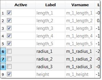
| 4. | In the work area, Active column, clear the radius_1, radius_2 and radius_3 checkboxes. |
| 5. | Go to the Specifications step. |
| 6. | In the work area, set the Mode to Hammersley. |
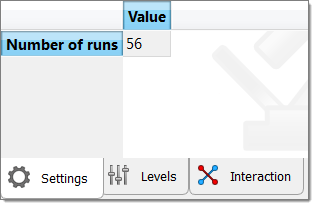
| 7. | In the Settings tab, change the Number of runs to 56. |
| 9. | Go to the Evaluate step. |
| 11. | Go to the Post processing step. |
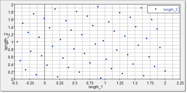
| 12. | To review a 2D scatter plot of the Hammersley DOE results, click the Scatter 2D tab. |
The image below illustrates a typical sampling of the Hammersley DOE with 56 Runs (Length 1 vs. Length 2).
| 13. | In the Explorer, right-click on the Hammersley DOE and select Copy Approach from the context menu. |
| 14. | In the Specifications step, change the number of runs to 12. |
| 15. | In the Evaluate step, click Evaluate Tasks. |
|
Using the 56 runs from the Hammersley DOE as an Input Matrix and the 12 runs from an additional Hammersley DOE as a Validation Matrix (does not apply to LSR), create a full quadratic LSR, full quadratic MLSM, HyperKriging, and Radial Basis Functions.
| 1. | In the Explorer, right-click and select Add Approach from the context menu. |
| 2. | In the HyperStudy - Add dialog, select Fit and click OK. |
| 3. | Go to the Select matrices step. |
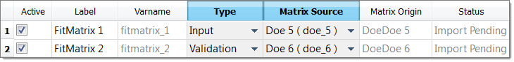
| 5. | In the HyperStudy - Add dialog, add two matrices. |
| 6. | Define FitMatrix 1 and FitMatrix 2, by selecting the options indicated in the image below from the Type and Matrix Source columns. |
| 8. | Go to the Specifications step. |
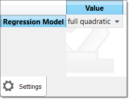
| 9. | In the work area, set the Mode to the appropriate Fit method. |
| 10. | In the Settings tab, set Regression Model to full quadratic for Least Square Regressions (LSR) and Moving Least Squares (MLSM). |
| 12. | Go to the Evaluate step. |
| 14. | Go to the Post processing step. |
| 15. | To review the error (and percentage) between the original output response and the approximation for each run of the input matrix, click the Residuals tab. |
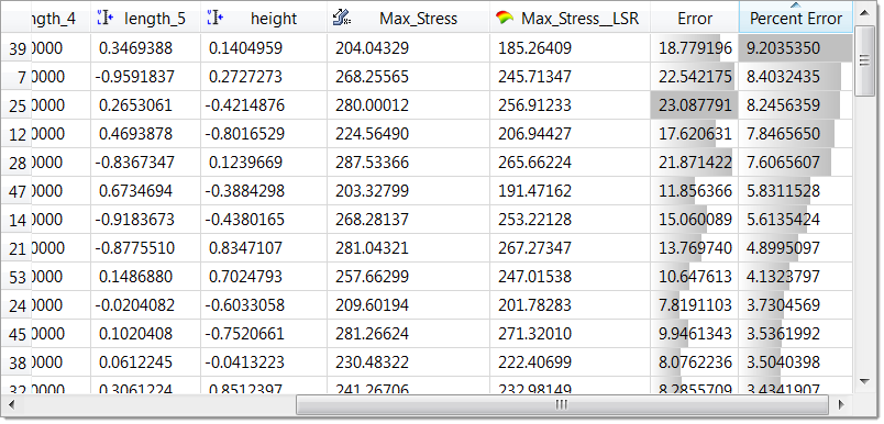
Residuals for Max_Stress, Least Square Regression.
| 16. | To review the diagnostics of the Fit study, click the Diagnostics tab. |
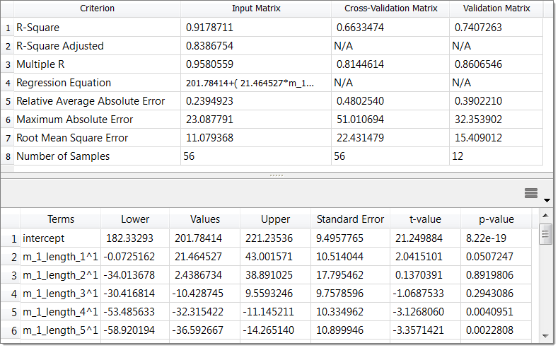
Diagnostics for Max_Stress, Least Square Regression.
|
The max percent of errors for the combined 56 + 12 run matrix (except for LSR, where this is not an option) are as shown below.
Method:
|
LSR
|
MLSM
|
HK
|
RBF
|
Order:
|
2nd order
|
2nd order
|
-
|
-
|
Max Disp:
|
-1.27
|
0.24
|
-0.00
|
0.00
|
Volume:
|
0.74
|
1.81
|
0.00
|
0.00
|
Max Stress:
|
-11.13
|
-4.39
|
-0.03
|
0.00
|
Percent of Error Value for Output Response Fits Obtained from Several Methods.
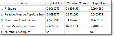
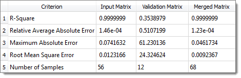
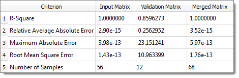
From this table, we can observe that any of the above methods give good results for linear output responses such as volume. For nonlinear output responses such as stress, RBF and MLSM accuracy is the best. We can also observe these findings from the diagnostic tables below.
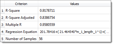
R-Square value for Max Stress is 0.92 in LSR, 0.996 in MLSM, 0.999 in HK and 1.0 in RBF.
LSR 2nd Order Diagnostics for Max_Stress
MLSM 2nd Order Diagnostics for Max_Stress
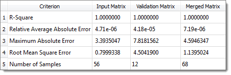
MLSM 2nd order Diagnostics for Volume
HyperKriging Diagnostics for Max_Stress
RBF Diagnostics for Max_Stress
|
See Also:
HyperStudy Tutorials


