HS-2000: DOE Method Comparison: Arm Model Study

In this tutorial you will:

•	Set up a Full Factorial DOE

•	Set up a 2-Level Fractional Factorial DOE

•	Set up a 3-Level Fractional Factorial DOE

•	Set up a Plackett-Burman DOE

•	Compare these methods in accuracy and efficiency

The files used in this tutorial can be found in <hst.zip>/HS-2000/. Copy the files from this directory to your working directory. The tutorial directory includes the following files:

arm_model.tpl	Template file
arm_model.optistruct.node.tpl	Grid coordinates template
arm_model.shp	Grid perturbation vector data for arm_model.optistruct.node.tpl

An arm model is used for this tutorial; the arm is clamped at one end and under an axial loading on the other end. It has been meshed and modeled in HyperMesh and analyzed using OptiStruct.

2000_crank

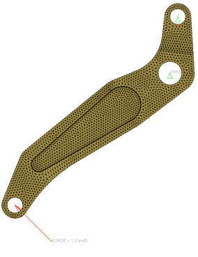
Concentrated load and boundary conditions

2000_crank2

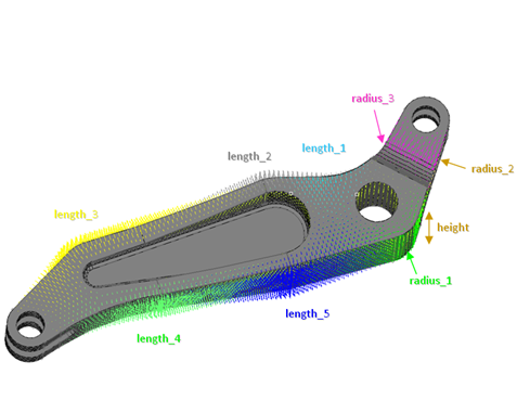
Shapes defined on the arm model

The design can change shape in nine different regions, as shown on the image above, and five output responses are of interest as detailed below.

Shape input variables	Length1:	Lower Bound = -0.5, Initial Bound = 0.0, Upper Bound = 2.0
	Length2:	Lower Bound = 0.0, Initial Bound = 0.0, Upper Bound = 2.0
	Length3:	Lower Bound = -1.0, Initial Bound = 0.0, Upper Bound = 1.0
	Length4:	Lower Bound = -1.0, Initial Bound = 0.0, Upper Bound = 1.0
	Length5:	Lower Bound = -1.0, Initial Bound = 0.0, Upper Bound = 1.0
	Radius1:	Lower Bound = -2.0, Initial Bound = 0.0, Upper Bound = 2.0
	Radius2:	Lower Bound = -0.5, Initial Bound = 0.0, Upper Bound = 1.0
	Radius3:	Lower Bound = -0.5, Initial Bound = 0.0, Upper Bound = 1.0
	Height:	Lower Bound = -1.0, Initial Bound = 0.0, Upper Bound = 1.0

Output Responses	Volume (Nominal design volume 1.7667e6 mm3)
	Max Von Mises Stress (Current design value = 195.29 MPa)
	Sum of stress on the model (983329 MPa)
	Nodal displacement of the node where the force is applied (mm) (1.411 mm)
	Nodal displacement of the extreme (lower end) node of the model (1.2555 mm)

Shape variables are created using HyperMesh’s morphing technology HyperMorph. In this tutorial we will start from an already morphed model. Moreover these shape variables are already exported for HyperStudy and a template is created.

1.	Start HyperStudy.

2.	To start a new study, click File > New from the menu bar, or click on the toolbar.

3.	In the HyperStudy – Add dialog, enter a study name, select a location for the study, and click OK.

4.	Go to the Define models step.

5.	Add a Parameterized File model.

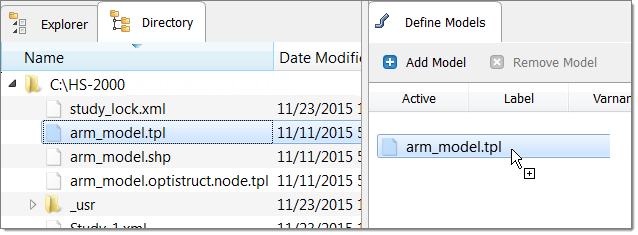
a.	From the Directory, drag-and-drop the arm_model.tpl file into the work area.

hs_2000_drag_drop_model

b.	In the Solver input file column, enter crank.fem. This is the name of the solver input file HyperStudy creates during any evaluation.

c.	In the Solver execution script column, select OptiStruct (os).

hs_2000_define models

6.	Click Import Variables. HyperStudy imports nine input variables from the arm_model.tpl resource file.

7.	Go to the Define Input Variables step.

8.	Review the input variable's lower and upper bound ranges.

9.	Go to the Specifications step.

1.	In the work area, set the Mode to Nominal Run.

2.	Click Apply.

3.	Go to the Evaluate step.

4.	Click Evaluate Tasks. An approach/nom_1/ directory is created inside the study directory. The approaches/nom_1/run__00001/m_1 directory contains the .res file, which is the result of the nominal run.

5.	Go to the Define Output Responses step.

In this step you will create three output responses: Max_Disp, Max_Stress, and Volume.

1.	Create the Max_Disp output response.

a.	From the Directory, drag-and-drop the crank.h3d file, located in approaches/nom_1/run_00001/m_1, into the work area.

b.	In the File Assistant dialog, set the Reading technology to Altair® HyperWorks® (Hyper3D Reader) and click Next.

c.	Select Multiple items at multiple time steps (readsim), then click Next.

d.	Define the following options, then click Next.

•	Set Subcase to Subcase 1 (SUBCASE1).

•	Set Type to Displacement (Grids).

•	Set Request (first - last) to N27099 - N40946.

•	Set Component to MAG.

hs-2000-max-disp-define

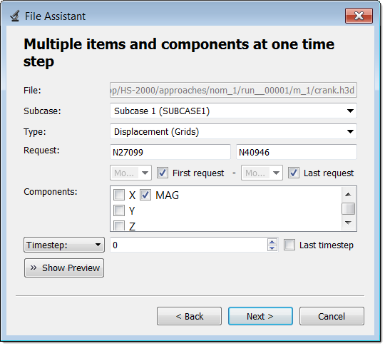
e.	Label the output response Max_Disp.

f.	Set Expression to Maximum.

hs-2000-max-disp-define2

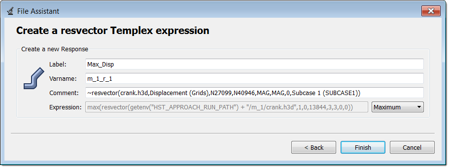
g.	Click Finish. The Max_Disp output response is added to the work area.

2.	Create the Max_Stress output response.

a.	From the Directory, drag-and-drop the crank.h3d file, located in approaches/nom_1/run_00001/m_1, into the work area.

b.	In the File Assistant dialog, set the Reading technology to Altair® HyperWorks® (Hyper3D Reader) and click Next.

c.	Select Multiple items at one time step (readsim), then click Next.

d.	Define the following options, then click Next.

•	Set Subcase to Subcase 1 (SUBCASE1).

•	Set Type to Element Stresses (3D).

•	Set Request (first-last) to E38257 - E94809.

•	Set Component to vonMises (2D & 3D).

e.	Label the output response Max_Stress.

f.	Set Expression to Maximum.

g.	Click Finish. The Max_Stress output response is added to the work area.

3.	Create the Volume output response.

a.	From the Directory, drag-and-drop the crank.out file, located in approaches/nom_1/run_00001/m_1, into the work area.

b.	In the File Assistant dialog, set the Reading technology to Altair® HyperWorks® (osmass.tpl) and click Next.

c.	Select Single item in a time series, then click Next.

d.	Define the following options, then click Next.

•	Set Type to OptiStruct Analysis.

•	Set Request to Out File.

•	Set Component to Volume.

e.	Label the output response Volume.

f.	Set Expression to First Element.

g.	Click Finish. The Volume output response is added to the work area.

4.	Click Evaluate Expressions to extract the output response values of each expression.

Parameter Screening DOE Setup

In this section, you will study the results from different parameter screening DOE's.

In the Full Factorial DOE, we will set the shape variables to two levels. Since full factorial runs all combinations of input variable values, we have no loss of information; however we have an expensive DOE. We will use this study as our reference to compare the loss of accuracy in the conclusions from other DOEs that are less expensive.

1.	In the Explorer, right-click and select Add Approach from the context menu.

2.	In the HyperStudy - Add dialog, select Doe and click OK.

3.	Go to the Specifications step.

4.	In the work area, set the Mode to Full Factorial.

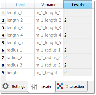
5.	Click the Levels tab, and change the number of levels for each input variable to 2.

Using nine shape variables with two levels gives a full factorial plan made of 512 runs (2^9).

hs_2000_full_fact

6.	Click Apply.

7.	Go to the Evaluate step.

8.	Click Evaluate Tasks.

9.	Go to the Post processing step.

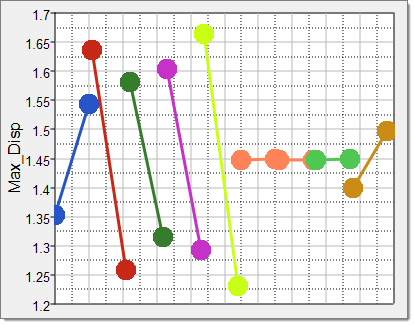
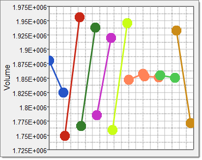
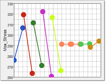
10.	Click the Linear Effects tab to view linear effect charts obtained from the Full Factorial DOE (512) runs.

From the main effects chart, it is understood that:

•	The three radius have almost no main effect on the output responses.

•	Lengths 2, 3, 4 and 5 have the same type of effect (direction and magnitude).

•	Length 1 and the height have the same direction of effect but are less important than the four other length variables.

It is also understood that going from the least influence to most influence on the max stress within the current ranges, the parameters can be sorted as:

radius 1

radius 2

radius 3

height

length 1

length 3

length 4

length 2

length 5

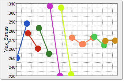
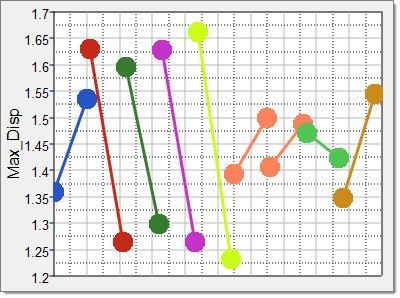
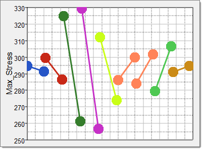
11.	Click the Interactions tab to plot the interactions between input variables.

Looking at the Max_stress output response, you can see that a number of interactions are very small. You can still find cases with a true interaction, such as the interaction of length 4 and length 5 illustrated in the image below. The effect of variable length 4 on output response Max_Stress is in the same direction whatever the value of length 5 is, but the effect (magnitude) is much more important when length 5 is large.

hs_2000_interactions1

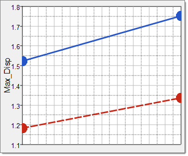
Length 1 and Length 2 on Max_Disp

hs_2000_interactions2

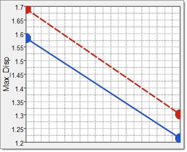
Length 2 and Height on Max_Disp

2000_c

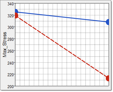
Length 4 and Length 5 on Max_Stress

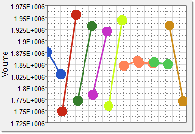
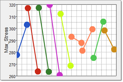
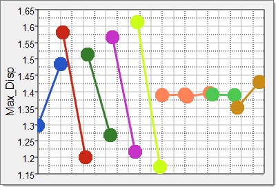
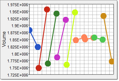
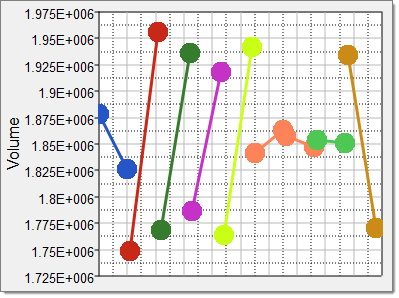
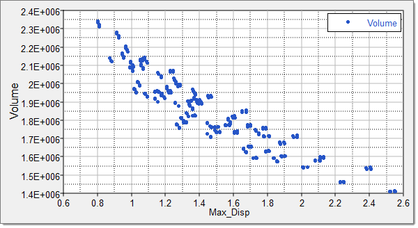
12.	Click the Scatter 2D tab to plot the results of the Full Factorial DOE (512).

13.	Click the Correlation tab, and select the cell for Max Disp vs. Volume (-0.92) to plot the linear correlation of -0.92 for Max Disp vs. Volume.

hs_2000_color_map1

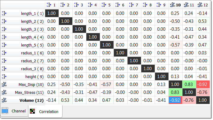
The scatter plot indicates a strong negative correlation between the volume of the part and its structural output responses.

hs_2000_plot1

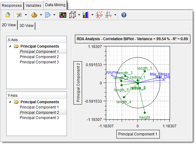
14.	Launch advanced post processing by clicking Tools > Post Processing from the menu bar.

15.	Open the Data Mining tool by click on the toolbar.

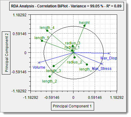
16.	On the toolbar, click and select RDA Analysis - Correlation Biplot from the list. HyperStudy displays a correlation biplot with input variables in green and output responses in blue.

2000_biplot

In this step you will set up a Fractional Factorial DOE with the same levels as the previous full factorial DOE. Using the nine input variables with two levels, without toggling ON any interaction, leads to a 16 runs Fractional factorial plan.

It is understood that the four length variables (2, 3 4 and 5) have a major effect on the model output responses. The three radii variables have a negligible effect on the volume and a small to medium effect on the displacement and stress.

It is also understood that length_1 has an opposed influence on the output responses compared to the other length shapes. It is seen that length and height have significant influences and we can focus on those variables for the rest of the studies. As for the three radii, we will set them to their nominal values to get the starting point.

1.	In the Explorer, right-click and select Add Approach from the context menu.

2.	In the HyperStudy - Add dialog, select Doe and click OK.

3.	In the Specifications step, set the Mode to Fractional Factorial.

4.	Click the Levels tab, and change the number of levels for each input variable to 2.

5.	Click Apply.

6.	Go to the Evaluate step.

7.	Click Evaluate Tasks.

8.	Go to the Post processing step.

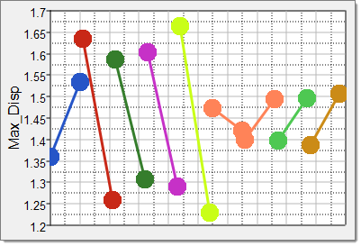
9.	Click the Linear Effects tab to view linear effect charts obtained from the 2 level Fractional Factorial DOE (16) runs.

$hs_2000_fract_fact1$	$hs_2000_fract_fact2$
$hs_2000_fract_fact3$

In this step you will set up a Fractional Factorial DOE with three levels. Using the nine input variables with three levels, without toggling ON any interaction, leads to a 27 runs Fractional factorial plan.

1.	In the Explorer, right-click and select Add Approach from the context menu.

2.	In the HyperStudy - Add dialog, select Doe and click OK.

3.	Go to the Specifications step.

4.	In the work area, set the Mode to Fractional Factorial.

5.	Click the Levels tab, and change the number of levels for each input variable to 3.

6.	Click Apply.

7.	Go to the Evaluate step.

8.	Click Evaluate Tasks.

9.	Go to the Post processing step.

10.

Click the Linear Effects tab to view linear effect charts obtained from the 3 level Fractional Factorial DOE (27) runs. The levels are: upper, lower and mean value. The initial value of the input variable is not considered (except of course when mean = initial). The linear effects chart indicates the following:

•	The 3 radii variables have a very small effect, except on max_stress where radius 1 and radius 2 can play a role.

•	Length 1 is opposed to the other length variables.

•	The use of 3 levels reveals that using only 2 levels can have hidden some interesting effects. Looking for example to max_stress vs. radius 1, if we consider only the 2 extreme levels, the main effect is rather small. If we now consider the intermediate level, we see a much larger influence.

$hs_2000_fract_fact3_1$	$hs_2000_fract_fact3_2$
$hs_2000_fract_fact3_3$

11.	Launch advanced post processing by clicking Tools > Post Processing from the menu bar.

12.	In the HyperStudy - Post Processing dialog, click on the toolbar.

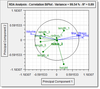
13.	On the toolbar, click and select RDA Analysis - Correlation Biplot from the list. HyperStudy displays a correlation biplot, which provides information on the negative strong correlation between volume and the other output responses.


RDA Analysis (correlation Biplot) this DOE on the left, the first DOE on the right

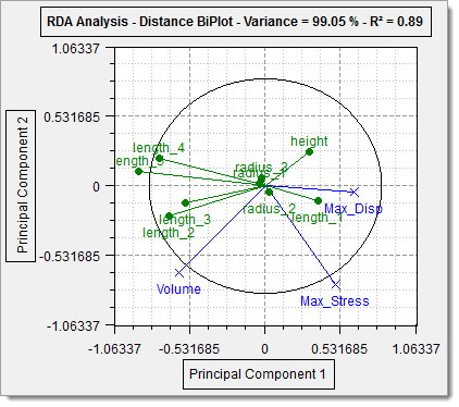
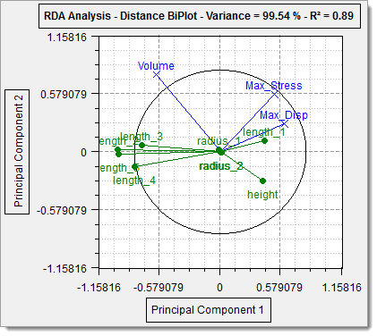
14.	On the toolbar, click and select RDA Analysis - Distance Biplot from the list. HyperStudy displays a distance biplot, which confirms the globally low impact of the radii variables on the model output responses.


RDA Analysis (Distance Biplot) this DOE on the left, the first DOE on the right

In this step you will set up a Plackett-Burman DOE which uses 2 levels for all the input variables. In this study, you will be using 9 variables,which will lead to a 12 run matrix.

1.	In the Explorer, right-click and select Add Approach from the context menu.

2.	In the HyperStudy - Add dialog, select Doe and click OK.

3.	Go to the Specifications step.

4.	In the work area, set the Mode to Plackett Burman.

5.	Click the Levels tab, and change the number of levels for each input variable to 2.

6.	Click Apply.

7.	Go to the Evaluate step.

8.	Click Evaluate Tasks.

9.	Go to the Post processing step.

10.	Click the Linear Effects tab to view linear effect charts obtained from the Plackett_Burman Doe (12 runs).

In the table below, relations and influences of input variables on the output response Sum of Stress is compared between the results obtained from the four DOE methods. Relations can be proportional, none or inverse. Influences can be high, medium, or low. As can be seen, despite few differences in these results, the conclusions from all the four methods is the same. In general, this trend is applicable, but note that depending on the application, there may be more or less differences in the results of DOE methods.

2000_conclusions

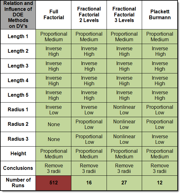
Comparison of Results (Relation and Influence of DV’s on Sum of Stresses) of Different DOE methods.

HS-2000: DOE Method Comparison: Arm Model Study

HS-2000: DOE Method Comparison: Arm Model Study

HS-2000: DOE Method Comparison: Arm Model Study

Shape input variables

Output Responses

Parameter Screening DOE Setup

See Also: