Continuing from tutorial HS-4000: Optimization Method Comparison: Arm Model Shape Optimization, we will perform stochastic studies using the same fitting function. You will run a stochastic study around the nominal point.
Before running this tutorial, you must complete tutorial Tutorial HS-4000: Optimization Method Comparison: Arm Model Shape Optimization or you can import the archive file HS-4000.hstx, available in <hst.zip>/HS-5000/.
In this stochastic study, you will be using a Hammersley distribution with 1000 runs. We defined all six input variables as random variables following a normal distribution with a variance of 0.1.
| 1. | In the Explorer, right-click and select Add Approach from the context menu. |
| 2. | In the HyperStudy - Add dialog, select Stochastic and click OK. |
| 3. | Go to the Select Input Variables step. |
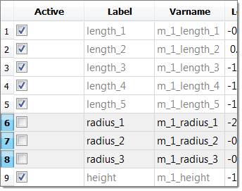
| 4. | In the Active column, clear the radius_1, radius_2 and radius_3 check boxes. |
| 5. | Click the Distributions tab. |
| 6. | In the Distribution column of the input variable Length 1, click  . . |
| 7. | Set Distribution Type to Normal_CoV. |
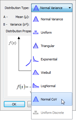 . .
| 8. | Set the Distribution Type to Normal_CoV for every active input variable. |
| 9. | Go to the Select Output Responses step. |
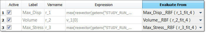
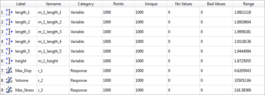
| 10. | Define Max_Disp, Volume and Max_Stress by selecting the options indicated in the image below from the Evaluate From column. |
| 11. | Go to the Specifications step. |
| 12. | In the work area, set the Mode to Hammersley. |
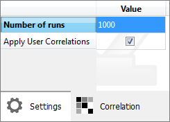
| 13. | In the Settings tab, change the Number of runs to 1000. |
| 15. | Go to the Evaluate step. |
| 16. | Click Evaluate Tasks to execute all 1000 runs and extract the results. |
| 17. | Go to the Post processing step. |
|
| 1. | Click the Distribution tab to review a histogram of the stochastic results. |
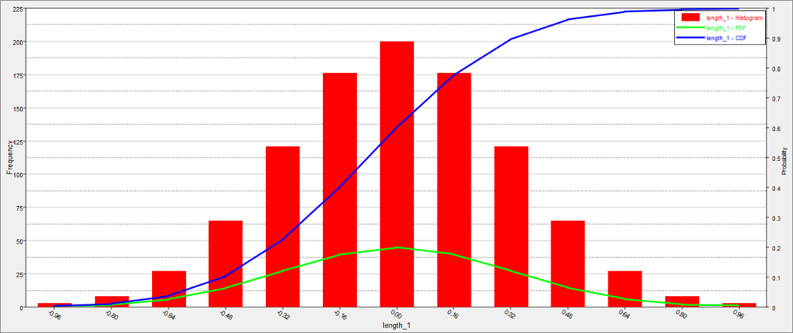
Using the Channel selector, select Length_1.
The chart shows three pieces of information about the distribution of values for the selected variable. The histogram uses the left axis, and represents the frequency count of the values. The probability distribution function (PDF) uses the right axis, and indicates the relative likelihood of the variable to take a particular value. A higher PDF value indicates that the values are more probable to occur. The cumulative distribution function (CDF) is another curve that uses the right axis. It is equal to the integral of the PDF. The value of the CDF indicates what percentage of the data falls below the value’s threshold. Note that the initial value of the CDF will always equal 0, and the final value of the CDF will always be 1.0. This is because all of the data will reside between the upper and lower bounds.
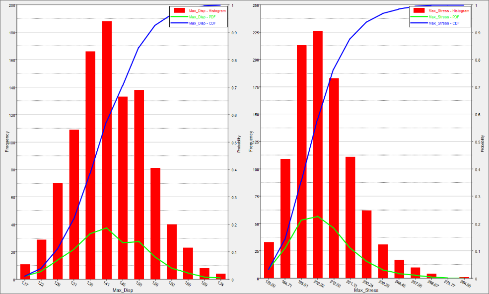
| 2. | Review the PDF and CDF of Max_Disp and Max_Stress by selecting Max_Disp and Max_Stress. |
Optional. To review the variables in separate histograms, click  . .
| 3. | Click the Integrity tab to review the statistics of the output responses around the nominal design. |
The column range can be useful to understand the spread of values in the data from the minimum to the maximum.
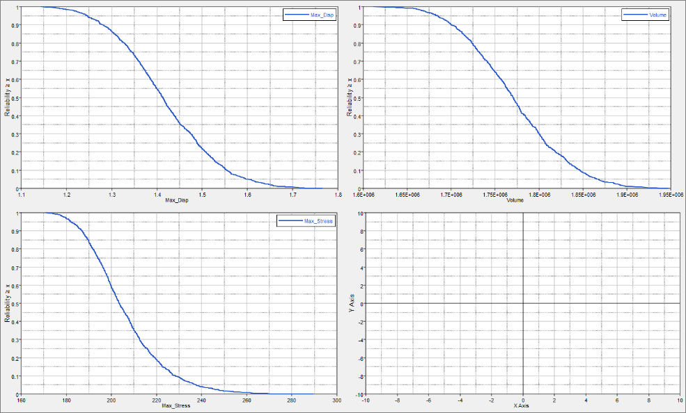
| 4. | Click the Reliability tab to estimate the Probability of failure for the output responses (probability for an output response to violate a user selected bound). |
| 6. | In the HyperStudy - Add dialog, add three reliabilities. |
| 7. | Define the three reliabilities by selecting the options indicated in the image below from the Response and Bound Type columns. |
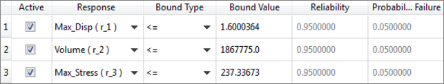
Study the effects of bounds on the reliability by entering different values in the Bound Value columns. The output response values for a standard probability range (95%) are illustrated in the image below. The values reported in the Reliability column can be observed on the reliability curves on the Reliability Plot tab. On the reliability curve, only 5% of the designs have a value above 1.6, which means 95% are below 1.6.
|
See Also:
HyperStudy Tutorials


