Continuing from Tutorial HS-3000: Fit Method Comparison: Approximation on the Arm Model, we will perform an optimization in this chapter and compare different methods in terms of efficiency and effectiveness.
Before running this tutorial, you must complete tutorial HS-3000: Fit Method Comparison: Approximation on the Arm Model or you can import the archive file HS-3000.hstx, available in <hst.zip>/HS-4000/.
For our baseline design (all shape variables set to 0.0) the corresponding output response values were:
Single Objective, Deterministic Optimization Study
In this section you will be comparing five single objective, deterministic optimization studies. You will be changing the number of shape variables used as well as the optimization method. During this section you will using the following optimization methods:
| • | Adaptive Response Surface Method |
| • | Sequential Quadratic Programming |
Using the conclusions of the different design of experiments, you will consider only six shape variables for the optimization and omit the three radii (we keep them fixed at their nominal values).
| 1. | In the Explorer, right-click and select Add Approach from the context menu. |
| 2. | In the HyperStudy - Add dialog, select Optimization and click OK. |
| 3. | Go to the Select Input Variables step. |
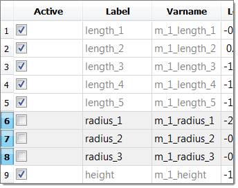
| 4. | In the work area, Active column, clear the radius_1, radius_2 and radius_3 check boxes. |
| 5. | Go to the Select Output Responses step. |
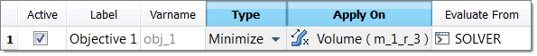
| 7. | In the HyperStudy - Add dialog, add one objective. |
| b. | Set Apply On to Volume. |
| 9. | Click the Constraints tab. |
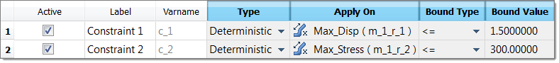
| 11. | In the HyperStudy - Add dialog, add two constraints. |
| 12. | Define Constraint 1 and Constraint 2 by selecting the options indicated in the image below from the Type, Apply On, Bound Type and Bound Value columns. |
| 14. | Go to the Specifications step. |
| 15. | In the work area, set the Mode to Adaptive Response Surface Method (ARSM). |
| Note: | Only the methods that are valid for the problem formulation are enabled. |
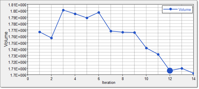
| 17. | Go to the Evaluate step. |
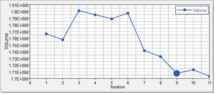
| 19. | Click the Iteration Plot tab to review the results of the optimization in an iteration plot. |
|
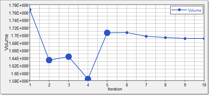
| 1. | Run a second single objective, deterministic Optimization study. Repeat steps 1 through 19 from Step 1: ARSM, Six Input Variables, Exact Solver, except in the Define Input Variables step, make sure all of the input variables are active. |
| 2. | Click the Iteration Plot tab to review the results of the optimization in an iteration plot. |
|
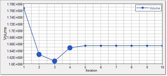
| 1. | Run a second single objective, deterministic Optimization study. Repeat steps 1 through 19 from Step 1: ARSM, Six Input Variables, Exact Solver, except in the Specifications step, set the Mode to Sequential Quadratic Programming (SQP). |
| 2. | Click the Iteration Plot tab to review the results of the optimization in an iteration plot. |
|

| 2. | Click the Constraint tab. |
| 4. | In the HyperStudy - Add dialog, add two constraints. |
| 5. | Define Constraint 1 and Constraint 2 by selecting the options indicated in the image below from the Type, Apply On, Bound Type and Bound Value columns. |

| 7. | Go to the Specifications step. |
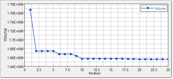
| 8. | In the work area, set the Mode to Sequential Quadratic Programming (SQP). |
| 10. | Go to the Evaluate step. |
| 12. | Click the Iteration Plot tab to review the results of the optimization in an iteration plot. |
|
| 2. | In the work area, set the Mode to Genetic Algorithm (GA). |
| 4. | Go to the Evaluate step. |
| 6. | Click the Iteration Plot tab to review the results of the optimization in an iteration plot. |
|
Reliability-Based Design Optimization Study
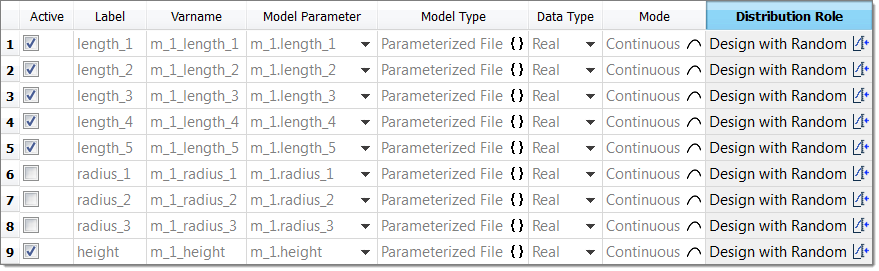
In this section, we will be searching for 95% reliability on the two optimization constraints (max_stress < 300 MPa and max_disp < 1.5 mm). We will be using fitting functions as opposed to the exact solver to evaluate the output responses. Among the approximations, we will be using RBF that is created with Hammersley DOE. As a result, we will be using the SORA method. We will continue using the six important input variables. They will all follow a normal distribution with a variance of 0.1.
| 2. | In the Select Input Variables step, click the Details tab. |
| 3. | For all six input variables, select Design with Random from the Distribution Role column as indicated in the image below. |
| 4. | Go to the Select Output Responses step. |
| 6. | In the HyperStudy - Add dialog, add one objective. |
| b. | Set Apply On to Volume (r_2). |
| c. | Set Evaluate From to Volume_RBF (r_2_fit_4). |
| 8. | Click the Constraint tab. |
| 10. | In the HyperStudy - Add dialog, add two constraints. |
| 11. | Define Constraint 1 and Constraint 2 by selecting the options indicated in the image below from the Type, Apply On, Bound Type, Bound Value, CDF Limit, and Evaluate From columns. |

| 13. | Go to the Specifications step. |
| 14. | In the work area, set the Mode to Sequential Optimization and Reliability Assessment (SORA). |
| 16. | Go to the Evaluate step. |
| 18. | Review the results of the Optimization in a table by clicking the Iteration History tab. |
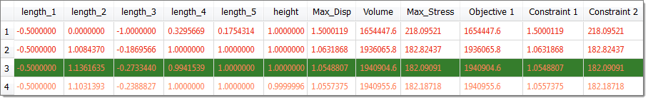
A deterministic optimum is found first. As you can see in iteration 1, the displacement is 1.50, which is the constraint bound. This design is not 95% reliable as required in this probabilistic Optimization study (95th percentile is 1.67). Then, SORA tightens the constraint bound for the deterministic Optimization to move into the safer region so that it is in the consecutive iterations, and the probabilistic constraint of 95% reliability can be met. As seen in iteration 3, the design that meets the 95% reliability is the one that has a max displacement of 1.05. Corresponding to this improvement, there is an increase in the objective value, which is volume of the part from 1.67E+06 mm3 to 1.94E+06 mm3.
|
Multi-Objective Optimization Study
In this section, we will be searching for the pareto front that minimizes both the volume and the maximum displacement, but under the constraint on the maximum stress (max_stress < 300 MPa). We will start from the nominal design. We are using MOGA with approximations to save time.
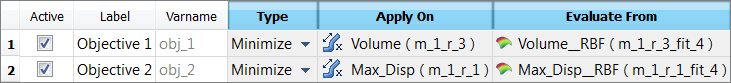
| 3. | In the HyperStudy - Add dialog, add two objectives. |
| 4. | Define Objective 1 and Objective 1 by selecting the options indicated in the image below from the Type, Apply On and Evaluate From columns. |
| 5. | Click the Constraint tab. |
| 7. | In the HyperStudy - Add dialog, add one constraint. |
| a. | Set Type to Deterministic. |
| b. | Set Apply On to Max_Stress. |
| d. | In Bound Value column, enter 300.00. |
| e. | Set Evaluate From to Max_Stress_RBF. |
| 10. | Go to the Specifications step. |
| 11. | In the work area, set the Mode to Multi-Objective Genetic Algorithm (MOGA). |
| 13. | Go to the Evaluate step. |
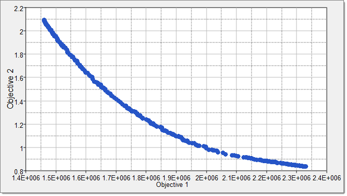
| 14. | Click Evaluate Tasks. HyperStudy stops MOGA after 50 iterations, and performs a total of 13317 analysises. The pareto front of the last iteration contains 408 points. |
| 15. | Go to the Post processing step. |
| 16. | Click the Iterations tab. |
| 17. | Review the Pareto front (objective versus objective). |
| a. | Using the Channel selector, select Objective 1 for the X Axis and Objective 2 for the Y Axis. |
| b. | Filter the entries to only include non-blank entries by right-clicking in the Best Step Major column and selecting Filter > 50 from the context menu. The optimal iterations display. |
| c. | Select all of the optimal designs by clicking the Iteration column. |
The Pareto front displays in the plot.
|
See Also:
HyperStudy Tutorials


