HS-4200: Material Calibration Using System Identification

The purpose of this tutorial is to introduce a method for characterizing parameters of a RADIOSS material law used for modeling elasto-plastic material. The characterization of a ductile aluminum alloy is studied. A RADIOSS simulation is performed to replicate an experimental tensile test. The parameters of the material law are determined to fit the experimental results.

HS-1506: Register a HyperMath Function provides an alternative method to setup this problem using a HyperMath function to measure the difference between two curves.

Description of the Model

A quarter of a standard tensile test specimen is modeled using symmetry conditions. A traction is applied to a specimen via an imposed velocity at the left-end.

The units are: mm, ms, g, N, MPa.

hs_1505_1

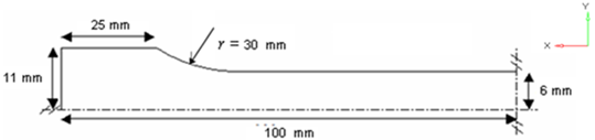
Geometry of the Tensile Specimen (One Quarter of the Specimen is Modeled)

hs_1505_2

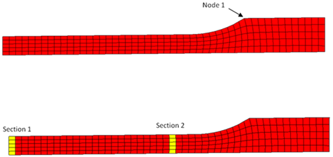
Sections of Node Saved for Time History

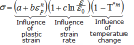
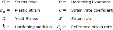
The material to be characterized is a 6063 T7 Aluminum: it has an isotropic elasto-plastic behavior which can be reproduced by a Johnson-Cook model without damage (RADIOSS Block Law2), defined as follows:

hs_1505_function

hs_4200_intro

In this study we define, as input variables, the parameters a, b, n, σmax (maximum stress) and the Young modulus. The stress-strain curve obtained by the experimental test is shown in the following image.

hs_1505_3

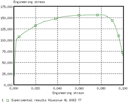
Engineering Stress Versus Engineering Strain Curve (Experimental Data)

For the simulation results, engineering strains will be obtained by dividing the displacement of node 1 by the reference length (75 mm), and engineering stresses will be obtained by dividing the force in section 1 by its initial surface (10.2 mm2).

hs_1505_4

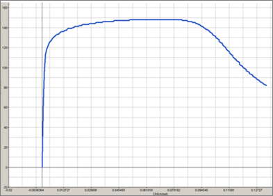
Engineering Stress Versus Strain Curve (Simulation Results)

In this tutorial, you will:

•	Create an input template from a RADIOSS data file using the HyperStudy Template Editor

•	Set up a study

•	Run a system identification optimization study

The sample base input template used in this tutorial can be found in <hst.zip>/HS-4200/. Copy the files TENSILE_TEST_0000.rad, TENSILE_TEST_0001.rad, and exper.xy from this directory to your working directory.

In this step, you can create the base input template in HyperStudy or use the base input template in the study directory.

1.	Start HyperStudy.

2.	From the menu bar, click Tools > Editor. The Editor opens.

3.	In the File field, navigate to your working directory and open the TENSILE_TEST_0000.rad file.

Note:

RADIOSS uses fixed fields of 20 characters for properties.

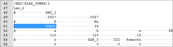
4.	In the Find area, enter /MAT/PLAS_JOHNS/1 and click . HyperStudy highlights /MAT/PLAS_JOHNS/1 in the TENSILE_TEST_0000.rad file.

hs_1505_find word

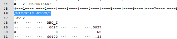
5.	Select E by starting at the beginning of row 51 and highlighting the first 20 fields.

Tip:	To assist you in selecting 20-character fields, press CTRL to activate the Selector (set to 20 characters) and then click the value.

hs_1505_e_field

6.	Right-click on the highlighted fields and select Create Parameter from the context sensitive menu.

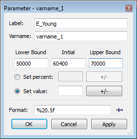
7.	In the Parameter Varname_1 dialog, enter E_Young in the Label field.

8.	Set the Lower Bound to 50000, the Initial Bound to 60400, and the Upper Bound to 70000.

9.	In the Format field, enter %20.5f.

hs_1505_design variable properties

10.

Click OK.

11.	Define four more variables using the information provided in the table below.

Note: Some of the initial values are different from the values in the original file.

Variable	Label	Lower Bound	Initial Value	Upper Bound	Format
a	a_PlasticityYieldStress	90	110	120	%20.5f
b	b_HardeningCoeff	100	125	160	%20.5f
n	n_HardeningExpo	0.1	0.2	0.3	%20.5f
sigmax	Sigma_Max	250	280	290	%20.5f

12.	Click Save.

13.	In the Save Template dialog, navigate to your working directory and save the file as TENSILE_TEST_0000.tpl.

14.	Close the Parameter Editor dialog.

1.	To start a new study, click File > New from the menu bar, or click on the toolbar.

2.	In the HyperStudy – Add dialog, enter a study name, select a location for the study, and click OK.

3.	Go to the Define models step.

4.	Add a Parameterized File model.

a.	From the Directory, drag-and-drop the TENSILE_TEST_0000.tpl file into the work area.

hs_4200_drag_drop_model

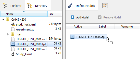
b.	In the Solver input file column, enter TENSILE_TEST_0000.rad. This is the name of the solver input file HyperStudy writes during any evaluation.

c.	In the Solver input file column, select RADIOSS (radioss).

d.	In the Solver input arguments column, enter -both at the end of $file. This argument runs the Starter, and the Engine of RADIOSS for the crash analysis. It also prevents the creation of the .h3d result file from animation files. X is the number of CPUs to use for the simulation.

5.	Define a model dependency.

a.	In the work area, right-click on the model and select Model resources from the context menu.

b.	In the Model Resource dialog, click Add Resource.

c.	In the Add - HyperStudy dialog, set Type to Normal and click OK.

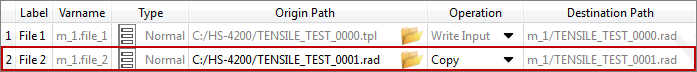
d.	In the Origin Path field, navigate to your working directory and open the TENSILE_TEST_0001.rad file.

e.	Set Operation to Copy.

f.	Click Close.

hs_4200_model_resource

6.	Click Import Variables. Five input variables are imported from the TENSILE_TEST_0000.tpl resource file.

7.	Go to the Define Input Variables step.

8.	Check the input variable's lower and upper bound ranges.

9.	Go to the Specifications step.

1.	In the work area, set the Mode to Nominal Run.

2.	Click Apply.

3.	Go to the Evaluate step.

4.	Click Evaluate Tasks. An approaches/nom_1/ directory is created inside the study directory. The approaches/nom_1/run__00001/m_1 directory contains the TENSILE_TESTT01 file, which stores the time history results of the simulation.

5.	Go to the Define Output Responses step.

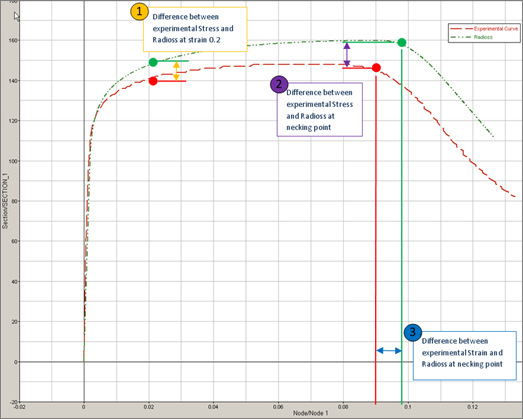
In order to fit the RADIOSS stress-strain curve to the experimental data we need to find a way to compare the two curves. In this tutorial we will only focus on three specific points on the curve.

Since damage is not modeled with this law, the comparison is not needed after the necking point.

•	Difference between experimental stress and RADIOSS at Strain equal 0.02 (1)

•	Difference between experimental strain and RADIOSS at Necking point (2)

•	Difference between experimental stress and RADIOSS at Necking point (3)

hs_6020_points

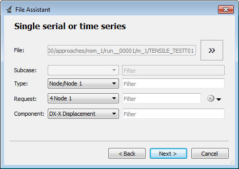
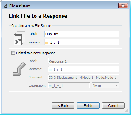
1.	Create a file source labeled Disp_sim.

a.	From the Directory, drag-and-drop the TENSILE_TEST01 file, located in approaches/nom_1/run_00001/m_1, into the work area.

b.	In the File Assistant dialog, set the Reading technology to Altair® HyperWorks® and click Next.

c.	Select Single item in a time series, then click Next.

d.	Define the following options, then click Next.

•	Set Type to None/Node 1.

•	Set Request to 4 Node 1.

•	Set Component to DX-X Displacement.

hs_1505_disp_sim

e.	Label the output response Disp_sim.

f.	Clear the Linked to a new Response checkbox.

g.	Click Finish

hs-4200-1

2.	Create a second file source labeled Force_sim by repeating step 1, except define the following options:

•	Set Type to Section/SECTION_2.

•	Set Request to 2 section 1.

•	Set Component to FT-Resultant Tangent Force.

3.	Add three output responses.

a.	Click Add Output Response.

b.	In the HyperStudy - Add dialog, add three output responses labeled: Radioss_Strain_0_2, Radioss_Stress_Necking, and Radioss_Strain_Necking.

4.	Define the Radioss_Strain_0_2 output response.

a.	In the Expression column of the output response Radioss_Strain_0_2, click .

b.	Click the Function tab.

c.	From the list of functions, select lininterp.

d.	Click Insert Varname. The function lininterp() appears in the Evaluate Expression field.

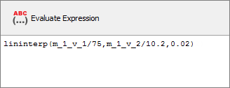
e.	In the Evaluate Expression field, enter (m_1_v_1/75,m_1_v_2/10.2,0.02) in the lininterp function.

This expression computes the Stress with respect to the Strain, at Strain equals 0.02.

hs_4200_expression

f.	Click Evaluate Expression.

Click OK.

5.	Define the Radioss_Stress_Necking output response.

a.	In the Expression column of the output response Radioss_Stress_Necking, click .

b.	In the Expression Builder, click the Functions tab.

c.	From the list of functions, select max.

d.	Click Insert Varname. The function max() appears in the Evaluate Expression field.

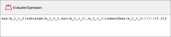
e.	In the Evaluate Expression field, enter (m_1_v_2[subrange(m_1_v_1,min(m_1_v_1),m_1_v_1[indexofmax(m_1_v_2)])])/10.2 in the max function.

This is the maximum of the force (m_1_v_2), which is trimmed between the min strain and the strain at the max value of Force, divided by 10.2 (surface) to obtain the stress.

hs_4200_expression2

f.	Click Evaluate Expression.

Click OK.

6.	Define the Radioss_Strain_Necking output response.

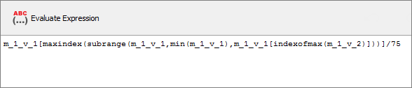
a.	In the Expression column of the output response Radioss_Strain_Necking, click .

b.	In the Evaluate Expression field, enter m_1_v_1[maxindex(subrange(m_1_v_1,min(m_1_v_1),m_1_v_1[indexofmax(m_1_v_2)]))]/75.

This is the displacement (m_1_v_1) at the max value of the force value, divided by 75 to obtain strain.

hs_4200_expression3

c.	Click Evaluate Expression.

Click OK.

1.	In the Explorer, right-click and select Add Approach from the context menu.

2.	In the HyperStudy - Add dialog, select Optimization and click OK.

3.	Go to the Select Input Variables step.

4.	Review the input variable's lower and upper bound ranges.

5.	Go to the Select Output Responses step.

6.	Add objectives.

a.	Click the Objectives tab.

b.	Click Add Objective.

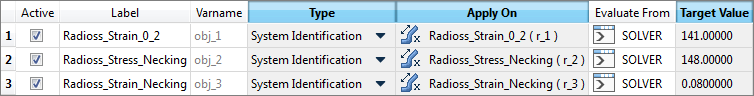
c.	In the Add-HyperStudy dialog, add three objectives labeled: Radioss_Strain_0_2, Radioss_Stress_Necking, Radioss_Strain_Necking.

d.	Define the three objectives by selecting the options indicated in the image below from the Type, Apply On, and Target Value columns.

e.	Click Apply.

hs_4200_objectives

7.	Go to the Specifications step.

8.	In the work area, set the Mode to Adaptive Response Surface Method (ARSM).

Note:

Only the methods that are valid for the problem formulation are enabled.

9.	Click Apply.

10.	Go to the Evaluate step.

11.	Click Evaluate Tasks to launch the Optimization.

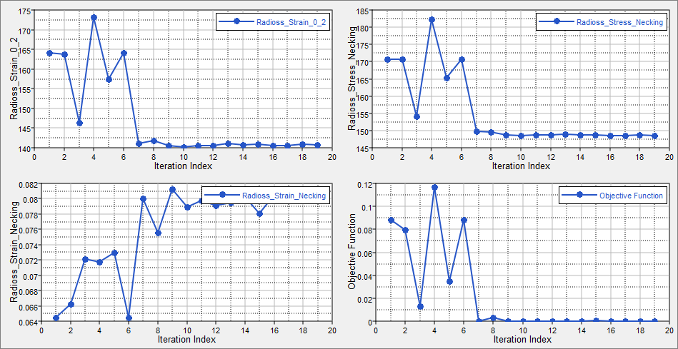
12.	Click the Iteration Plot tab.

Using the Channel selector, select the three objectives from and the Objective Function Value. Activate multi-plot to see the each channel in its own plot.

The first three selections are the actual values used in the system identification optimization problem. Observe their objective history to see that their values indeed approach their respective target values. The final plot is the scalar objective which is used in the system identification problem; a normalized sum of the squares difference between the actual and target objective values. Note that the value of this combined function has been reduced through the optimization.

6020_plot

HS-4200: Material Calibration Using System Identification

HS-4200: Material Calibration Using System Identification

HS-4200: Material Calibration Using System Identification

Description of the Model

Variable

Label

Lower Bound

Initial Value

Upper Bound

Format

See Also: