In this tutorial you will learn how to use the objective function type MaxMin through a frequency maximization application.. The sample base input template plate.tpl can be found in <hst.zip>/HS-4410/ and copied to your working directory.
The objective is to maximize the minimum frequency of the first five modes of a plate. The input variables are the thickness of each of the three components, defined in the input deck via the PSHELL card. The thickness should be between 0.05 and 0.15; the initial thickness is 0.1 (shown below). The optimization type is size.
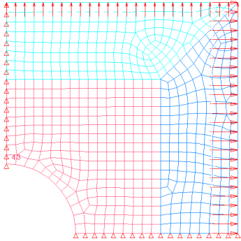
Figure 1: Double symmetric plate model
| 2. | To start a new study, click File > New from the menu bar, or click  on the toolbar. on the toolbar. |
| 3. | In the HyperStudy – Add dialog, enter a study name, select a location for the study, and click OK. |
| 4. | Go to the Define models step. |
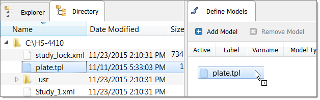
| 5. | Add a Parameterized File model. |
| a. | From the Directory, drag-and-drop the plate.tpl file into the work area. |
| b. | In the Solver input file column, enter plate.fem. This is the name of the solver input file HyperStudy writes during any evaluation. |
| c. | In the Solver execution script column, select OptiStruct (os). |

| 6. | Click Import Variables. One input variable is imported from the plate.tpl resource file. |
| 7. | Go to the Define Input Variables step. |
| 8. | Review the input variable's lower and upper bounds ranges. |
| 9. | Go to the Specifications step. |
|
| 1. | In the work area, set the Mode to Nominal Run. |
| 3. | Go to the Evaluate step. |
| 4. | Click Evaluate Tasks. An approaches/nom_1/ directory is created inside the study directory. The approaches/nom_1/run__00001/m_1 sub-directory contains the plate.out file, which is the result of the nominal run, and will be used during the Optimization. |
| 5. | Go to the Define Output Responses step. |
|
| 1. | Click Add Output Response. |
| 2. | In the HyperStudy - Add dialog, add five output responses. |
| 3. | In the Expression column of Response 1, click  . . |
| 4. | In the Expression Builder, click the File Sources tab. |
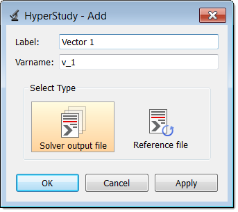
| 6. | In the HyperStudy - Add dialog, add one Solver output file. |
| 7. | In the File column of Vector 1, click . |
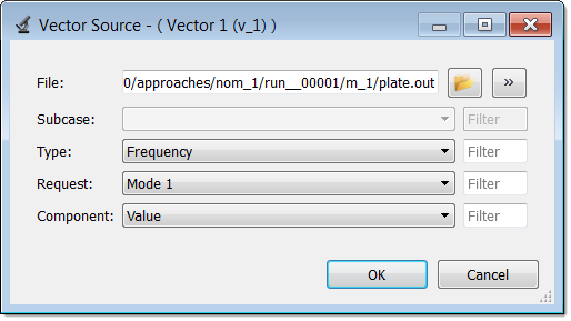
| 8. | In the Vector Source dialog, navigate to the approaches/nom_1/run__00001/m_1 directory and open the plate.out file. |
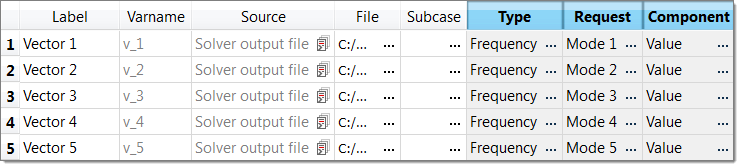
| 9. | Define Vector 1 as the volume of the plate by selecting the options indicated in the following image from the Type, Request, and Component fields. |
| 11. | Click Insert Varname. The expression v_1[0] appears in the Evaluate Expression field. |
| 13. | Repeat steps 3 through 12 for Response 2 through Response 5. Define each Vector by selecting the options indicated in the image below from the Type, Request, and Component columns. |
| 14. | Click Evaluate Expressions to extract the output response values. |
This completes the study setup. You can now proceed to the desired study type (DOE, Optimization, or Stohastic study).
|
| 1. | In the Explorer, right-click and select Add Approach from the context menu. |
| 2. | In the HyperStudy - Add dialog, select Optimization and click OK. |
| 3. | Go to the Select Input Variables step. |
| 4. | Review the input variable's lower and upper bound ranges. |
| 5. | Go to the Select Output Responses step. |
| 7. | In the HyperStudy - Add dialog, add five objectives. |
| 8. | Define Objective1 through Objective 5 by selecting the options indicated in the image below from the Apply On column. |
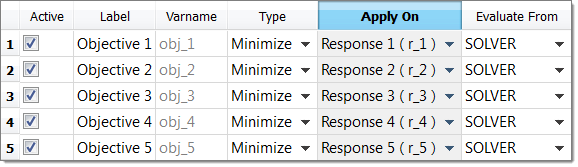
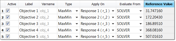
| 9. | Maximize the minimum for all five objectives by selecting MaxMin from the Type column. |
| 10. | In the study Setup, Define Output Responses step, copy the values for all five output responses in the Value column. |
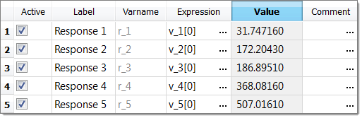
| 11. | In the Optimization, Select Output Responses step, paste the values into the Reference Value column. |
| 13. | Go to the Specifications step. |
| 14. | In the work area, set the Mode to Adaptive Response Surface Method (ARSM). |
| Note: | Only the methods that are valid for the problem formulation are enabled. |
| 16. | Go to the Evaluate step. |
|
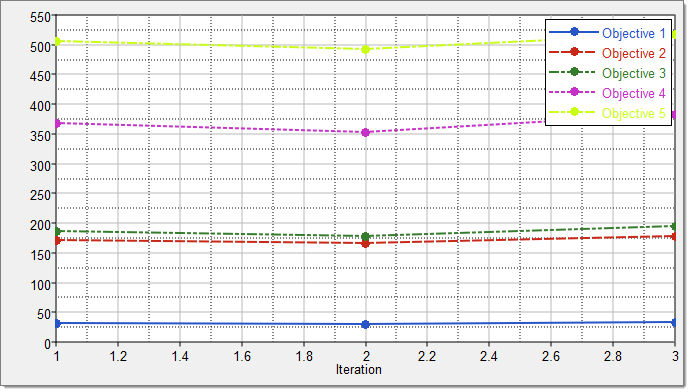
| 1. | Click the Iteration Plot tab to monitor the progress of the Optimization iteration. |
| 2. | Using the Channel selector, select all five objectives. The Optimization iteration history of Objective 1 through Objective 5 is plotted. |
|
See Also:
HyperStudy Tutorials


