The inclusion matrix feature passes an already existing set of data to the running process. In this tutorial, the data created from a DOE is passed to an optimization problem which re-uses the data. This promotes efficient design exploration practices: an optimization using a direct solver call can still be done in combination with a DOE to study the system without any loss of data. This example focuses on the competing objectives in the design of a cantilever ibeam.
The files used in this tutorial can be found in <hst.zip>/HS-4450/. Copy the files from this directory to your working directory.
| 2. | To start a new study, click File > New from the menu bar, or click  on the toolbar. on the toolbar. |
| 3. | In the HyperStudy – Add dialog, enter a study name, select a location for the study, and click OK. |
| 4. | Go to the Define models step. |
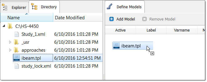
| 5. | Add a Parameterized File model. |
| a. | From the Directory, drag-and-drop the ibeam.tpl file into the work area. |
| b. | In the Solver input file column, enter ibeam.py. This is the name of the solver input file HyperStudy writes during any evaluation. |
| c. | In the Solver execution script column, select Python (py). |

| 6. | Click Import Variables. Four input variables are imported from the ibeam.tpl resource file. |
| 7. | Go to the Define Input Variables step. |
| 8. | Review the input variable's lower and upper bounds ranges. |
| 9. | Go to the Specifications step. |
|
| 1. | In the work area, set the Mode to Nominal Run. |
| 3. | Go to the Evaluate step. |
| 4. | Click Evaluate Tasks. An approaches/nom_1/ directory is created inside the study directory. The approaches/nom_1/run__00001/m_1 sub-directory contains the output.hstp file, which is the result of the nominal run, and will be used during the Optimization. |
| 5. | Go to the Define Output Responses step. |
|
| 1. | Create the Iy output response for the y-axis moment of inertia. |
| a. | From the Directory, drag-and-drop the output.hstp file, located in approaches/nom_1/run_00001/m_1, into the work area. |
| b. | In the File Assistant dialog, set the Reading technology to Altair® HyperWorks® (HstReaderPdd) and click Next. |
| c. | Select Single item in a time series, then click Next. |
| d. | Define the following options, and then click Next. |
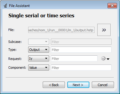
| e. | Label the output response Iy. |
| f. | Set Expression to Maximum. |
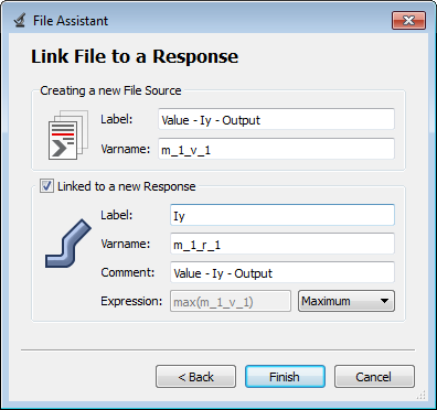
| g. | Click Finish. The Iy output response is added to the work area. |
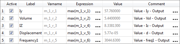
| 2. | Create four more output responses by repeating step 1, except change the component assigned to each output response to the following. |
Output Response
|
Component
|
Volume
|
Vol
|
IZ
|
Iz
|
Displacement
|
d
|
Frequency1
|
Freq
|
| 3. | Click Evaluate Expressions to extract output response values. |
| 4. | Click OK. This complete the study setup. |
|
| 1. | In the Explorer, right-click and select Add Approach from the context menu. |
| 2. | In the HyperStudy - Add dialog, select Doe and click OK. |
| 3. | Go to the Specifications step. |
| 4. | In the work area, set the Mode to Hammersley. |
| 5. | In the Settings tab, verify that the Number of runs is 17. |
| 7. | Go to the Evaluate step. |
| 9. | Go to the Post processing step, and click the Pareto Plot tab. |
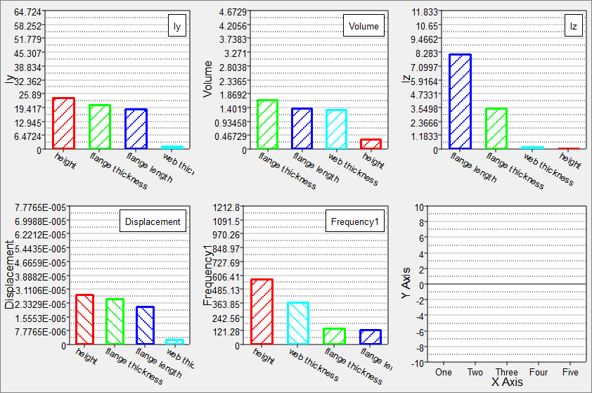
Enable multi-plot and select all of the output responses in the Channel selector. In the options menu, ensure that Effects based on all variables is enabled.
A Pareto Plot shows the ranked influence of the input variables on the output response. For example, for the y-axis moment of the inertia, height has the largest influence and web thickness has the least. In contrast, for the z-axis moment of inertia, the flange length and flange thickness are the most influential variables. The size of the bar indicates the magnitude of the influence, and the hashed line’s slope indicates the sign of the effect: positive or negative. For example, increasing the height will increase Iy, but it will decrease displacement.
|
| 1. | In the Explorer, right-click and select Add Approach from the context menu. |
| 2. | In the HyperStudy - Add dialog, select Optimization and click OK. |
| 3. | Go to the Select Input Variables step. |
| 4. | Review the input variable's lower and upper bound ranges. |
| 5. | Go to the Select Output Responses step. |
| 7. | In the HyperStudy - Add dialog, add two objectives labeled. |
| 8. | Define the two objectives by selecting the options indicated in the image below. |
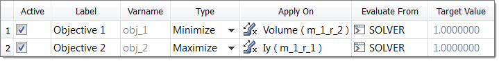
| 10. | Go to the Specifications step. |
| 11. | In the work area, set the Mode to Global Response Surface Method (GRSM). |
| Note: | Only the methods that are valid for the problem formulation are enabled. |
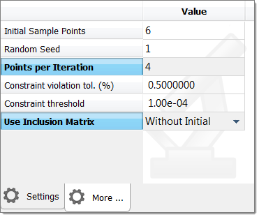
| 12. | Click the More tab and define the following settings: |
| • | Set Points per Iteration to 4. |
| • | Set Use Inclusion Matrix to Without Initial. |
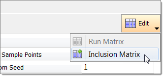
| 13. | Import run data from the Doe using an Inclusion Matrix. |
| a. | Click Edit > Inclusion Matrix from the top, right corner of the work area. |
| b. | In the Edit Inclusion Matrix dialog, click Import Values. |
| c. | In the Import Values dialog, select Approach Evaluation Data and click Next. |
| d. | Select the approach to Doe 1 and click Next. |
| f. | Review the imported run data and click OK. |
| 15. | Go to the Evaluate step. |
| 16. | Click Evaluate Tasks to launch the Optimization. |
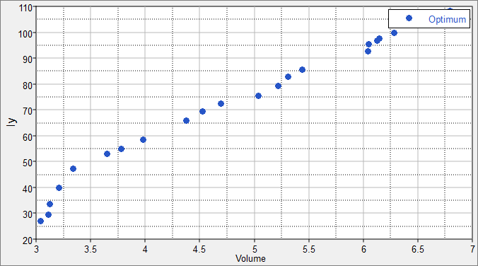
| 17. | Go to the Post Processing step, and click the Optima tab. |
Observe the non-dominated front of designs. These points represent the trade-off between the objective of minimizing volume and maximizing the y-axis moment of inertia. In the plot, it is evident that as the moment of inertia increases, the volume increases as well. This curve represents the trade-off of the best available designs given the competing objective requirements.
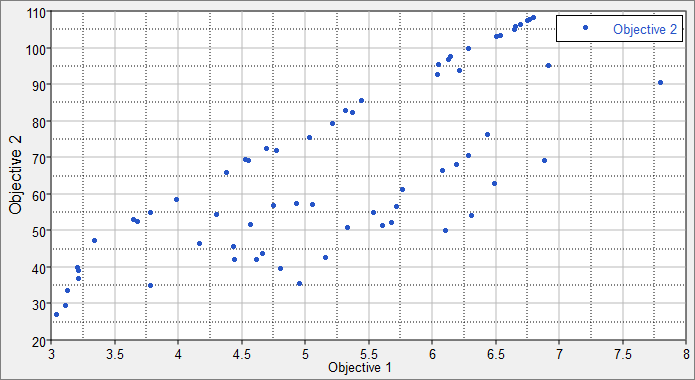
| 18. | Go to the 2D Scatter tab, and plot the objectives along same axes shown in the Optima plot. |
This plot shows all of the runs from the optimization. When comparing the scatter and Optima plots, note that the Optima plot contains only the subset of runs which are non-dominated. A dominated design is a design for which both objectives could be improved. A non-dominated design is one in which one objective may only be improved at the expense of another.
|


