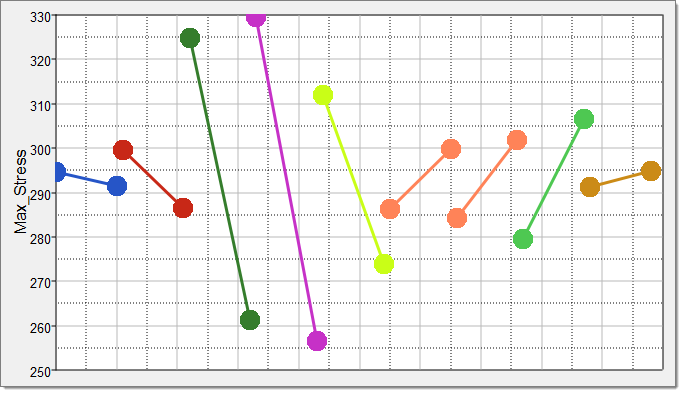
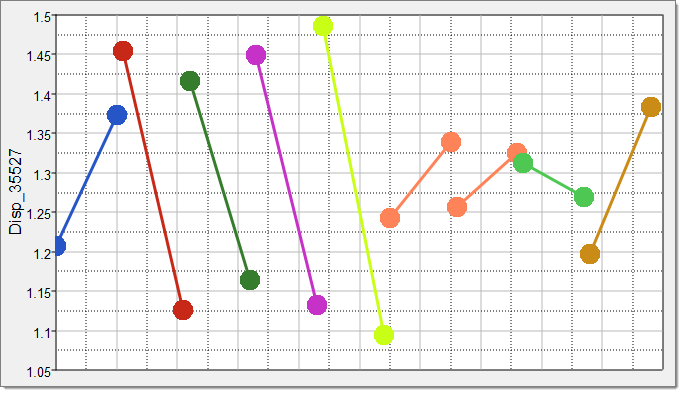
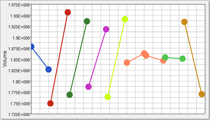
In this study, we want to analyze the volume, the displacement at the force application (node 35527), and the maximum stresses. Three output responses will be created.
| 1. | Click Add Output Response. |
| 2. | In the HyperStudy - Add dialog, add three output responses and label them Max_Stress, Disp_35527, and Volume. |
| 3. | In the Expression column of the output response Max_Stress, click  . . |
| 4. | In the Expression Builder, click the Functions tab. |
| 5. | From the list of functions, select max. |
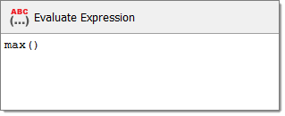
| 6. | Click Insert Varname. The function max() appears in the Evaluate Expression field. |
| 7. | From the list of functions, select readsim. |
| 9. | In the readsim - Builder dialog, navigate to the approaches/nom_1/run__00001/m_1 directory and open the crank.res file. |
| 10. | From the Subcase, Type, Request, and Component fields, select the options indicated in the image below. |
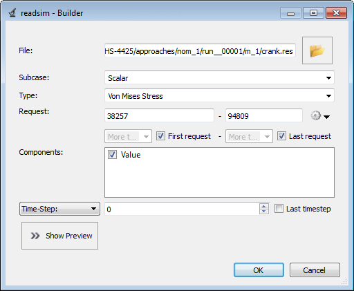
| 11. | Click OK. The expression reads: max(readsim(getenv("HST_APPROACH_RUN_PATH") + "/m_1/crank.res", "Scalar", "Von Mises Stress", "firstrequest", "lastrequest", "{Value}", 0)). This expression returns the max value of the stress vector. |
| 13. | In the Expression column of the output response Disp_35527, click . |
| 14. | In the Expression Builder, click the File Sources tab. |
| 15. | Click Add File Source. |
| 16. | In the HyperStudy - Add dialog, add one Solver output file. |
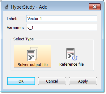
| 17. | In the File column of Vector 1, click . |
| 18. | In the Vector Source dialog, navigate to the approaches/nom_1/run__00001/m_1 directory and open the crank.res file. |
| 19. | Define Vector 1 as the magnitude of displacement at node 35527 by selecting the options indicated in the image below from the Subcase, Type, Request, and Component fields. |
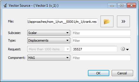
| Note: | Because there is only a single value in this vector, HyperStudy inserts a [0] after v_1, thereby choosing the first (and only) entry in the vector. |
| 23. | Repeat steps 13 through 17 for the output response Volume. |
| 24. | In the Vector Source dialog, navigate to approaches/nom_1/run__00001/m_1 directory and open the crank.out file. |
| 25. | Define Vector 2 as the volume of the crank model by selecting the options indicated in the image below from the Type, Request, and Component fields. |
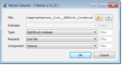
| Note: | Because there is only a single value in this vector, HyperStudy inserts a [0] after v_2, thereby choosing the first (and only) entry in the vector. |
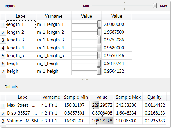
| 29. | Click Evaluate Expressions to extract the output response values. |
|