HS-4420: Optimization Study of a Spherical Impactor

This tutorial demonstrates how to perform an advanced study that has both size and shape input variables on a RADIOSS finite element model.

The sample base input template can be found in <hst.zip>/HS-4420/. Copy the files impactor.hm, impactor_0000.rad, and impactor_0001.rad from this directory to your working directory.

The steps taken in this tutorial demonstrate how to analyze the input variables in order to identify the most important variables and how to do an optimization. The objective of the optimization is to minimize the maximum acceleration of the impactor while keeping maximum displacement lower than 16 mm.

In this tutorial, you will:

•	Create a base input template from a RADIOSS input file using the HyperStudy Editor

•	Set up a study

•	Run a DOE study (screening DOE)

•	Post process DOE results in order to define the most important variables and reduce the number of variables (screening)

•	Create a new DOE in order to create an approximation

•	Create an approximation

•	Run an optimization study based on the approximation created

This model simulates the dynamic impact of a sphere with an initial velocity on a box. There are eight variables: four size variables, which are four box thickness, and four shapes variables.

hs_6010_size_var

Size variables

hs_6010_shapes

Shapes variables

1.	Start HyperMesh Desktop.

2.	In the User Profiles dialog, change the user profile to RADIOSS (Block100).

3.	From the menu bar, click File > Open > Model.

4.	In the Open Model dialog, open the impactor.hm file. The impactor.hm database has the RADIOSS analysis setup, and the shapes have already been created. Now you have to export the shapes variables, so they have included in the template file.

5.	From the Tool page, click Shape.

hs_4420_shape_panel

6.	Go to the desvar subpanel.

7.	Switch single desvars to multiple desvars.

hs_4420_desvar_subpanel

8.	In the initial value= field, enter 0.

9.	In the lower bound= field, enter -1.

10.	In the upper bound= field, enter 1.

11.	Click the shapes selector.

hypermesh_shape_selector

12.	Select all of the shapes.

13.	Click select.

14.	Click create. A shape design variable is created for each shape.

15.

Optional.

•	If you would like to animate or visualize the shapes, click animate.

•	In the Deformed panel, click linear or modal to animate the shape variables in the graphics area.

•	While the shape is animating, you can adjust the animation speed by moving the slider as indicated in the image below.

hs_3070_animate

16.	Go to the export subpanel.

17.	For analysis code, select HyperStudy.

18.	For sub-code, select Radioss51.

19.	In the File field, enter impactor.shp.

hs_4420_export_panel

20.	Click export as.

21.	In the Save As dialog, navigate to your working directory and save the file as impactor.shp. HyperMesh writes the following files:

impactor.radioss51.node.tpl	Grid coordinates template.
impactor.shp	Grid perturbation vector data read by impactor.radioss51.node.tpl.

22.	Exit HyperMesh Desktop.

1.	Start HyperStudy.

2.	From the menu bar, click Tools > Editor. The Editor opens.

3.	In the File field, open the impactor_0000.rad file.

4.	Right-click anywhere in the editor and select Select Nodes > /NODE from the context menu. All of the /NODE cards in the impactor_0000.rad file highlight.

hs-4420-2

5.	Right-click on the highlighted cards and select Include Shape from the context menu.

6.	In the Shape Template dialog, open the impactor.radioss51.node.tpl file. The shape variables are now created and the grid has been replaced by the parameter file (which contains the grid parameterized by the shapes) exported during step 1.

7.	Locate the shape variable prop_external_skin.

8.	Select the thickness value for prop_external_skin, as indicated in the image below. In a RADIOSS deck, each field within a card is 20 characters long.

Tip:	To assist you in selecting 20-character fields, press CTRL to activate the Selector (set to 20 characters) and then click the value. HyperStudy highlights 20 fields.

hs_4420_variable1

9.	Right-click on the highlighted fields and select Create Parameter from the context menu.

10.	In the Parameter - varname_1 dialog, Label field, enter th_external_skin.

11.	Set the Lower bound to 1.0, the Initial to 1.0, and the Upper bound to 2.0.

12.	Set the Format to %20.5f.

13.

Click OK.

hs_4420_variable1_create

14.	Define three more input variables for thickness using the information provided in the table below.

Input Variable	Label	Lower Bound	Initial Value	Upper Bound	Format
prop_internal_skin	th_internal_skin	1.0	1.0	2.0	%20.5f
prop_external_flange	th_external_flange	1.0	1.0	2.0	%20.5f
prop_internal_flange	th_internal_flange	1.0	1.0	2.0	%20.5f

15.	Click Save.

16.	In the Save Template dialog, navigate to your working directory and save the file as impactor.tpl.

17.	Close the Editor.

1.	To start a new study, click File > New from the menu bar, or click on the toolbar.

2.	In the HyperStudy – Add dialog, enter a study name, select a location for the study, and click OK.

3.	Go to the Define models step.

4.	Add a Parameterized File model.

a.	From the Directory, drag-and-drop the impactor.tpl file into the work area.

hs_4420_drag_drop_model

b.	In the Solver input file column, enter impactor_0000.rad. This is the name of the starter input file HyperStudy creates from the parameterization, and the name of the Engine file.

c.	In the Solver execution script column, select RADIOSS (radioss).

d.	In the Solver input arguments column, enter -both -nproc 4 after $file.

5.	Define a model dependency.

a.	In the work area, right-click on the model and select Model resources from the context menu.

b.	In the Model Resource dialog, click Add Resource.

c.	In the Add - HyperStudy dialog, set Type to Normal and click OK.

d.	Define the resource.

•	In the Origin Path field, navigate to your working directory and open the impactor_0001.rad file.

•	Set Operation to Copy.

e.	Click Close.

hs_4420_model_resource

6.	Click Import Variables. Eight input variables are imported from the impactor.tpl resource file.

7.	Go to the Define Input Variables step.

8.	Review the lower and upper bound ranges of the input variables.

9.	Go to the Specifications step.

1.	In the work area, set the Mode to Nominal Run.

2.	Click Apply.

3.	Go to the Evaluate step.

4.	Click Evaluate Tasks. An approach/nom_1/ directory is created inside the study directory. The the approaches/nom_1/run__00001/m_1 sub-directory contains the impactorT01 file, which is the result of the nominal run.

5.	Go to the Define Output Responses step.

In this study, we want to analyze the maximum acceleration and the maximum displacement observed by the box. This study is a function of the time; we need to extract the maximum of each output response vector over time.

1.	Create a file source for time.

a.	From the Directory, drag-and-drop the impactorT01 file, located in approaches/nom_1/run_00001/m_1, into the work area.

b.	In the File Assistant dialog, set the Reading technology to Altair® HyperWorks® and click Next.

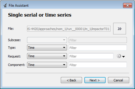
c.	Select Single item in a time series, then click Next.

d.	Define the following options, then click Next.

•	Set Type to Time.

•	Set Request to Time.

•	Set Component to Time.

hs_4420_vector1

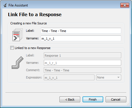
e.	Clear the Linked to a new Response checkbox.

f.	Click Finish

hs_4420_vector1_2

2.	Create a second file source for impactor acceleration along the Z axis. Repeat step 1, except define the following options:

•	Set Type to Node/TH_node_sphere.

•	Set Request to 4206 rigid_sphere_4206.

•	Set Component to AZ-Z Acceleration.

3.	Create a third file source for impactor displacement along the Z axis. Repeat step 1, except define the following options:

•	Set Type to Node/TH_node_sphere.

•	Set Request to 4206 rigid_sphere_4206.

•	Set Component to DZ-Z Displacement.

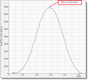
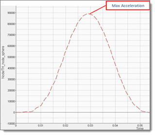
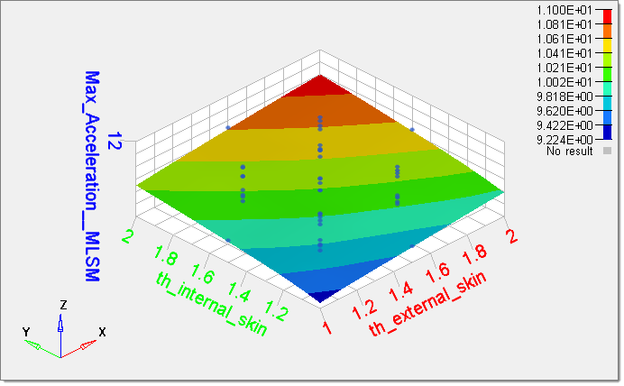
You have finished creating all of the result vectors for the Max_Acceleration output response. As you can see from the graph on the left-hand side below, it has some noise. To eliminate the noise, you will use a filter and work on the filtered output response as seen from the graph on the right-hand side below.

4420_max_accel

4420_max_accel2

4.	Add two output responses.

a.	Click Add Output Response.

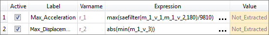
b.	In the HyperStudy - Add dialog, add two output responses labeled: Max_Acceleration and Max_Displacement.

5.	Define the Max_Acceleration output response.

a.	In the Expression column of the output response Max_Acceleration, click .

b.	In the Expression Builder, click the Functions tab.

c.	From the list of functions, select saefilter. This function will apply a filter to the acceleration vector.

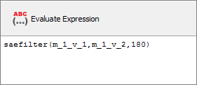
d.	Click Insert Varname. The function saefilter(,,) appears in the Evaluate Expression field.

You can now add the time vector and the acceleration vector as arguments to the function, with a class parameter of 180.

e.	In the Evaluate Expression field, enter (m_1_v_1,m_1_v_2,180) in the saefilter function.

hs_4420_max_acceleration

f.	To calculate the max of the expression, add the max function to the beginning of the expression.

The expression should read: max(saefilter(m_1_v_1,m_1_v_2,180)).

g.	To express the result in G, divide the max of the expression by 9810.

The expression should read: max(saefilter(m_1_v_1,m_1_v_2,180)/9810).

Click OK.

6.	Define the Max_Displacement output response.

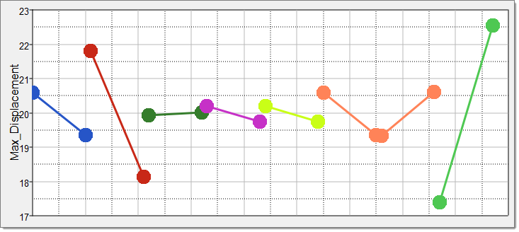
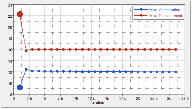
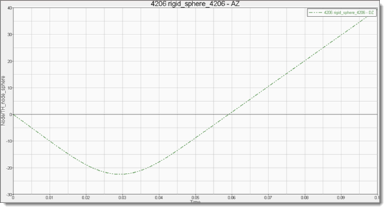
a.	Optional. Plot the displacement with respect to the time, to obtain the curve illustrated below:

4420_curve

b.	In the Expression column of the output response Max_Displacement, click .

c.	In the Expression Builder, click the Functions tab.

d.	From the list of functions, select abs.

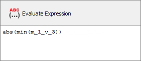
e.	Click Insert Varname. The function abs()appears in the Evaluate Expression field.

f.	From the list of functions, select min.

g.	Click Insert Varname. The expression should now read, abs(min()).

h.	In the Evaluate Expression field, enter m_1_v_3 in the min function.

hs_4420_max_disp

Click OK.

7.	Click Evaluate to extract the output response values of each expression.

hs_4420_evaluate_expression

The model has 8 variables which may lead to high computation times for direct optimization or even for creating a response surface.

We will reduce the number of actual input variables by running a screening experiment. A full factorial experiment with 8 factors at 2 levels will require 28 (256) runs and with 3 levels, it will increase to 6561 runs. We will try to screen out some input variables by first doing a Plackett-Burman screening DOE.

1.	In the Explorer, right-click and select Add Approach from the context menu.

2.	In the HyperStudy - Add dialog, select DOE and click OK.

3.	Go to the Specifications step.

4.	In the work area, set the Mode to Plackett-Burman.

5.	Click Apply.

6.	Go to the Evaluate step.

7.	Click Evaluate Tasks to execute the run matrix and extract the output responses for all of the runs. HyperStudy runs 12 simulations in Plackett Burman mode, therefore the evaluation will take some time.

8.	Go to the Post processing step.

1.	Click the Linear Effects tab to review the linear effects.

4420_post1

4420_post2

This above figures show:

•	As the four thickness variables increase, maximum acceleration increases.

•	As the four thickness variables increase, maximum displacement decreases.

You can remove the Radius variable since it does not contribute to any of the output responses. To reduce the number of input variables, remove the variables listed below, as they are less influential than other variables.

•	th_external_flange

•	th_internal_flange

•

Radius

2.	To launch the advanced Post Processing tool for data mining, click Launch Post Processing. HyperStudy loads the current result file (.data extension).

3.	To open the Data Mining tool, click .

4.	To perform a PCA data analysis, click on the toolbar.

5.	Review the Distance BiPlot and a the Correlation BiPlot.

6.	To plot the regression coefficient in a histogram, click . The highest values indicate the most influential variables. This supports the conclusion above, that the variables that have the least effect are th_external_flange, Radius, length_external and width_external.

4200_regression

In a classic DOE analysis, we analyze the main effects, but we also analyze the interactions between input variables. In this tutorial, we have done a Screening DOE which does not allow for evaluating the interactions.

For the rest of the study, you will only use the following variables:

•	th_external_skin

•	th_internal_skin

•	length_external

•	width_external

•	length_internal

The other variables will be defined to their initial value.

Since this optimization is based on response surfaces, a central composite experiment will be used, which will create a 2nd order response surface.

1.	In the Explorer, right-click and select Add Approach from the context menu.

2.	In the HyperStudy - Add dialog, select Doe and click OK.

3.	Go to the Select Input Variables step.

4.	In the Active column, clear the th_external_flange, th_internal_flange and Radius checkboxes.

hs_4420_excludevar

5.	Go to the Specifications step.

6.	In the work area, set the Mode to Central Composite.

7.	Click Apply.

8.	Go to the Evaluate step.

9.	Click Evaluate Tasks to execute the run matrix and to extract the output responses.

10.	Go to the Post processing step.

Other points will be used to check the quality of the approximation. The points will be defined by a new DOE. In this DOE study, a Latin Hypercube of 10 runs will be used.

1.	Add a third Doe to the study by repeating Step 8: Run a DOE Study for Approximation, except in the Specifications step, set the Mode to Latin HyperCube and change the Number of runs to 10.

1.	In the Explorer, right-click and select Add Approach from the context menu.

2.	In the HyperStudy - Add dialog, select Fit and click OK.

3.	Go to the Select matrices step.

4.	Click Add Matrix.

5.	In the HyperStudy - Add dialog, add two matrices.

6.	Define FitMatrix1 and FitMatrix2 by selecting the options indicated in the following image from the Type and Matrix Source columns.

hs_4425_select_matricies

7.	Click Import Matrix.

8.	Go to the Select Input Variables step.

9.	Review the input variables and output responses. The th_external_flange, th_internal_flange, and Radius input variables are still inactive.

10.	Go to the Specifications step.

11.	In the work area, set the Mode to Moving Lease Squares (MLSM).

12.	For Order, select 2.

13.	Click Apply.

14.	Go to the Evaluate step.

15.	Click Evaluate Tasks.

16.	Go to the Post processing step.

17.	To assess the accuracy of the regression equations, click the Residuals and Diagnostics tab.

18.	To review the output response curves and surfaces, click the Trade-Off tabs.

In the Trade-Off 3D tab, use the Channel selector to plot input variables and output responses. The values for the input variables which are not plotted are modified in the top frame (Inputs). Move the sliders in the Value column to modify the other input variables, while studying the output response throughout the design space.

hs_4420_tradeoff

1.	In the Explorer, right-click and select Add Approach from the context menu.

2.	In the HyperStudy - Add dialog, select Optimization and click OK.

3.	Go to the Select Input Variables step.

4.	In the Active column, clear the th_external_flange, th_internal_flange and Radius checkboxes. These input variables contribute less effects than the other variables.

5.	Go to the Select Output Responses step.

6.	Click Add Objective.

7.	In the HyperStudy - Add dialog, add one objective.

8.	Define the objective.

a.	Set Type to Minimize.

b.	Set Apply On to Max_Acceleration (r_1).

c.	Sethe Evaluate From to Max_Acceleration__MLSM (r_1_fit_1).

4200_objx

9.	Click the Constraint tab.

10.	Click Add Constraint.

11.	In the HyperStudy - Add dialog, add one constraint.

12.	Define the constraint.

a.	Set Apply On to Max_Displacement (r_2).

b.	Set Bound Type to <= (less than or equal to).

c.	For Bound Value, enter 16.

d.	Set Evaluate From to Max_Displacement__MLSM (r_2_fit_1).

4200_constraints

13.	Click Apply.

14.	Go to the Specifications step.

15.	In the work area, set the Mode to Genetic Algorithm (GA).

Note:

Only the methods that are valid for the problem formulation are enabled.

16.	In the Settings tab, change the Constraint violation tol. to 0.0.

17.	Click Apply.

18.	Go to the Evaluate step.

19.	Click Evaluate Tasks to optimize the design that minimizes the maximum acceleration while keeping the displacement of node 35527 smaller than 16.

20.	Click the Iteration Plot tab to monitor the Optimization iteration.

4200_iterplot

21.	Click the Iteration History tab to review a table of each iteration. The iterations that do not respect the constraint are displayed red, the optimal design is displayed green.

You have now determined the best design evaluated from the approximation. You can launch a solver run with the following input variables to check if the solution found by the approximation is close to the solver results.

1.	In the Explorer, click Define Input Variables from the study Setup section.

2.	Change the initial values to the values defined in the table below.

Variable Name	Optimum Value
th_external_skin	2.00
th_internal_skin	2.00
th_external_flange	1.00
th_internal_flange	1.00
Radius	0.00
length_external	-1.00
width_external	-0.81
length_internal	-1.00

3.	Go to the Evaluate step.

4.	Click Evaluate Tasks.

5.	Go to the Define Output Responses step.

6.	Compare the optimum solution evaluated from the approximation to the same design evaluated by the solver.

Note:

Due to the use of different solver versions, results may vary.

Output Responses	Approximation	Solver
Max_Acceleration	12.465	12.667 (1.62% error)
Max_Displacement	15.999	15.839 (1.00% error)

HS-4420: Optimization Study of a Spherical Impactor

HS-4420: Optimization Study of a Spherical Impactor

HS-4420: Optimization Study of a Spherical Impactor

Input Variable

Label

Lower Bound

Initial Value

Upper Bound

Format

See Also: