|
»Click here to display Table of Contents«
|

HyperStudy Terminology |

|

|

|

|
|
HyperStudy Terminology |
|
|
|

|
|
»Click here to display Table of Contents«
|
HyperStudy Terminology |
|
|
|
|
|
HyperStudy Terminology |
|
|
|
|
Used as a convergence criterion in optimization algorithms. The process has converged when there are two consecutive designs for which the absolute change in the objective function is less than the absolute convergence value, times the initial objective function value. Convergence is reached under the condition that the allowable violation has not been exceeded by any constraint in the last design.
ANOVA (Analysis of Variance) is a useful technique for estimating error variance and for determining the relative importance of various factors.
In HyperStudy, the ANOVA is performed only on Least Square Approximations. The ANOVA is plotted as the Percentage contribution of each input variable, the interactions and the Error.
The following quantities are computed in the process of performing the ANOVA:
| • | DoF - Degrees of freedom, Number of terms in the approximation |
| • | SS - Sum of squares |
| • | MSS - Mean sum of squares (MSS = SS/DoF) |
| • | % - Percentage contribution |
| • | Fo - F0 value (F0 = MSS(Variable)/MSS(Error)) |
A study approach is a certain set of steps taken to study the mathematical model of a design. In HyperStudy, there are four approaches: DOE, fit, optimization and stochastic. Each approach serves a different design study purpose and the required steps for each approach may be unique. For example, you can use the DOE approach if you need to learn the main factors affecting your design, but you need to use the optimization approach if you want to find the design that achieves the design objectives while satisfying design requirements.
Expression that relates the output response of interest back to the input variables that were varied. HyperStudy provides polynomial least square regressions, Moving Least Squares Method, and HyperKriging to define approximations. An approximation is only as good as the levels (number of designs) used when performing the study. For example, a two-level parameter only has a linear relationship in the regression. Higher order polynomials can be introduced by using more levels.
Note: Using more levels results in more runs. |
Response surface, Surrogate model, or Transfer of function are often used as synonyms for Approximation.
A variable which can take a set of values that are strings which cannot be ranked numerically. For example, the color of a car may be blue, red, or yellow.
Bounds on output response functions of the system that need to be satisfied for the design to be acceptable.
Constraint screening is the process by which the number of output responses in the optimization problem is trimmed to a representative set. This set of retained output responses captures the essence of the original design problem while keeping the size of the optimization problem at an acceptable level. Constraint screening utilizes the fact that constrained output responses that are a long way from their bounding values (on the satisfactory side) or that are less critical (i.e. for an upper bound more negative and for a lower bound more positive) than a given number of constrained output responses of the same type, within the same designated region and for the same subcase, will not affect the direction of the optimization problem and therefore can be removed from the problem for the current design iteration.
Constraints must not be violated by more than this value in the converged design.
For a controlled interaction, parallel lines indicate that the two displayed parameters have no interaction. Crossed lines indicate an interaction between the two parameters. It is common for interactions to change when aliasing has occurred.
System parameters that can be changed to improve the system performance in the chosen output response. Its value is under the control of the designer. Examples: Gauges, shape, material distribution, material properties.
Interactions between controlled and uncontrolled variables. This is independent of the design type selected (for either) and is always available when conducting a study with uncontrolled variables. If there is a significant interaction, it is recommended that the study be repeated with the uncontrolled variables as controlled variables.
A technique used to generate Fit quality metrics from only an input data set; no validation set is required. HyperStudy uses a k-fold cross-validation scheme, which means input data is broken into k groups. For each group, the group's data is used as a validation set for a new Fit using only the other group's data.
Plots the cumulative probability of each input variable or output response value. It increases from 0.0 to 1.0.
A collection of data obtained from the evaluation of HyperStudy approaches. It is presented in tabular form where each row represents a design, and columns represent the variables and output responses.
Where the datasets are stored. HyperStudy uses the depot to retrieve the datasets of a previously run study.
Often used to represent a parameter study using a Design of Experiments. The DOE is actually the way the input variable combinations for the study are chosen. It is a method to perform a parameter study with a minimum number of designs (experiments) to obtain as complete as possible information about the design space. The opposite would be a full-factorial analysis (complete design matrix), with all possible input variable combinations selected. A parameter study is used to study the behavior of design in the given design space.
HyperStudy provides the following Designs of Experiments:
| • | Full factorial |
| • | Fractional factorial |
| • | Latin Hypercube |
| • | Hammersley |
| • | Central Composite Design |
| • | Plakett-Burman |
| • | Box-Behnken |
A variable whose value is subject to uncertainty due to manufacturing, operating condition or environmental factors (among other possibilities). During the design process, mean values for random input variables can be controlled. As such, while there is uncontrolled randomness in the variable value, the distribution is fixed about a designable mean value. Examples include part dimensions such as length, width, or height. In a Stochastic approach Design with Random leads to a truncated sampling using the upper and lower bounds.
Diagnostics helps to assess the accuracy of the response surface. The diagnostics in HyperStudy contains the following information:
| • | R^2 (R-square) and R^2-adjusted value |
| • | Confidence limits on each regression coefficient (Least squares regression) |
| • | Root mean square |
| • | Relative maximum |
| • | Absolute maximum difference |
Design input (variable) thats value is changed to cause a change in the output (response).
One that satisfies all of the constraints.
A fit approach is one of the study approaches available in HyperStudy. It is used to construct a mathematical function that best fits to a dataset imported from a DOE or a Stochastic approach. This function then can be used instead of the exact solvers in other approaches to save computational resources.
Sorts the different designs (solver runs) into up to 25 buckets. It plots the number of runs in a bucket (frequency) over the input variable or output response.
Special form of interpolation to build an approximation. It is a special case of Moving Least Squares Method with a high closeness of fit.
Inclusion Matrix
An optional set of known data provided to a HyperStudy approach. This data is not collected during the evaluation phase and is known in advance; this is in contrast to the data in the Run matrix, which is typically collected at the time of a run. How the information is used varies from approach to approach and method to method.
One that violates one or more constraint functions.
System parameter that influences the system performance in the chosen output response.
An input variable is a property of the study. It is an object that is varied by the study based on certain rules. You can associate an input variable to a particular model parameter. Two input variables cannot be associated with the same model parameter. An input variable does not always need to be associated to a model parameter. Input variables can be linked within or across models.
Used as a convergence criterion in optimization algorithms. An optimization has converged when there are two consecutive designs for which the change in each input variable is less than this value, times the difference between its bounds; and this value, times the absolute value of its initial value (simply this value if the initial value is zero). Convergence is reached under the condition that the allowable violation has not been exceeded by any constraint in the last design.
Method to build an approximation using polynomial expressions. The coefficients of the polynomial are determined by a least squares regression.
The number of levels per variable to be considered, depends on the level of non linearity in the problem. Two levels are sufficient for a linear model and three levels are needed for a quadratic model.
Shows the effect of a change in the level of an input variable on the output response. Linear effects are shown in table and plot format. In a plot, if the line is horizontal, it implies that the input variable has no effect on the output response of interest. As the line becomes more vertical, the effect is larger. A positive slope indicates that changing the parameter value will result in a direct change to the output response. A negative slope indicates an inverse association.
An optimization will stop, regardless of convergence, when this number of iterations has been completed.
A model parameter is a property of the model being studied. It could be the mass of a body or the coordinates of a point, for example. The model parameter should not be confused with the input variable in a study. HyperStudy assigns a unique name to each model parameter which always begins with the model varname. In the example m_1.component1.mass, the m_1 label indicates that the model parameter is a property of the study model whose varname is m_1.
Method to build an approximation. As opposed to a simple Least Squares Regression, the coefficients of the approximation are dependent on the input variables.
An optimization problem that has multiple objective functions as opposed to a single objective function. With MOO, the objective is to find the trade-off curve between conflicting objectives (Pareto Front). This trade-off curve is a collection of nondominated designs. Usually the computational effort required to solve MOO problems are significantly more compared to single objective optimization problems.
A design that is better than all others in at least one criteria.
Any output response function of the system to be optimized. The output response is a function of the input variables. Examples: Mass, Stress, Displacement, Frequency, etc.
Mathematical procedure to determine the best possible design for a set of given constraints by changing the input variables in a defined manner.
Set of input variables along with the minimized (maximized) objective function that satisfies all of the constraints.
Measurement of system performance. Examples are: weight, volume, displacement, stress, strain, reaction forces, and frequency.
Set of Pareto optimal solutions (non-dominated designs)
Analysis to find the probability with which a design will fail. In addition to the output responses, the result of an analysis is a probability with which it has the value obtained by an analysis. The problem to solve is: How reliable is my design? Compare the result of a probability analysis with the requirements.
Methods are:
| • | Analytical methods (FORM – First order reliability method; SORM – Second order reliability method, etc.). |
| • | Sampling based methods (Monte-Carlo methods). |
HyperStudy provides sampling based methods to perform probabilistic analyses.
Plots the probability of each input variable or output response value. It is always between 0.0 and 1.0.
A parameter whose value is subject to uncertainty due to uncontrollable factors such as operating conditions (among others). A random parameter is not designable; its mean value is fixed. The randomness of the parameter has an effect on the design’s performance, however the nature of the randomness cannot be controlled during the design process. Examples include environmental conditions such as temperature or humidity.
Used as a convergence criterion in optimization algorithms. An optimization has converged if the relative (percentage) change in the objective function is less than this value for two consecutive designs. Convergence is reached under the condition that the allowable violation has not been exceeded by any constraint in the last design.
As opposed to worst-case based design, reliability based design considers the distribution of the input variables and noise factors. Each measure (constraint, target) must be met by x% of the designs. The optimization problem solved is to minimize weight under the constraint that x% of all designs can fail, or constraints must be met by (100-x)% designs. This can lead to considerable weight savings versus a worst-case based design. Six-sigma design is a design where one in one million designs fail. Example: Space shuttle - One in 250 starts failed. HyperStudy has the capability for performing reliability-based design by combining an optimization study with a stochastic study.
The difference between the output response value from the solver and the output response value from the response surface is the error, or the residual. The residual plot can be used to determine which runs are generating more error in the model.
A robust design is insensitive to small design changes. It minimizes the variations in performance and puts design on a predefined target.
There are two types of robust design:
| • | Variation in noise factors. |
| • | Variation in input variables. |
HyperStudy has the capability for performing robust design by combining an optimization study with a stochastic study.
A run matrix contains a summary of run data.
Method by which the designs (input variable combinations) that will be analyzed are determined. Amongst the many sampling methods are:
| • | Simple random sampling |
| • | Latin Hypercube |
| • | Hammersley sampling |
Of these three methods, Hammersley gives the most even distribution of sampling points (designs) and is therefore the most efficient.
The extent to which the uncontrolled (noise) variables influence the output response. This is similar to the main effects for controlled input variables.
The result of a stochastic analysis is not a deterministic output response value, but an output response value with a distribution. It is a method of probabilistic analysis. Instead of using a single value for input variables and noise factors, each has a distribution.
This is a procedure to fit a set of output responses to a set of target values by modifying a set of input variables. Optimization is used to accomplish this. The objective function is formulated as a least squares formula.
See Approximation.
The T-value is a measure of the quality of a polynomial approximation. It is computed using:
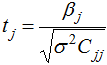
where ![]() is the corresponding regression coefficient,
is the corresponding regression coefficient, ![]() is the diagonal coefficient of the matrix
is the diagonal coefficient of the matrix ![]() . The value
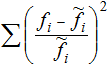
. The value ![]() is computed from:
is computed from:
![]()
with:
SSE – Sum of error squares of predicted versus actual value.
n – Number of samples (runs) in the model.
p – Number of regression terms.
The T-value has the same sign as the regression coefficient. Its value is undefined (infinite) if the error is zero. A regression coefficient is important for the model if ![]() , where
, where ![]() . The value
. The value ![]() is looked up from the t-distribution with parameters
is looked up from the t-distribution with parameters ![]() and n-p-1. The larger the T-value, the more important the coefficient is for an accurate approximation.
and n-p-1. The larger the T-value, the more important the coefficient is for an accurate approximation.
Uncontrolled is the interactions dialog for the uncontrolled parameters in the study.
System parameters that cannot be changed, but that influence the system performance in the chosen output response. Its values are not under the control of the designer. Examples are: loads, BC's, environmental conditions, and sometimes material.
Output responses defined in the study setup and not used during the optimization neither as objective function nor as constraint.
Parameter study to verify the quality of a response surface. This study is executed in addition to the study that is used to produce the approximation in the first place.