|
»Click here to display Table of Contents«
|

Problem Formulation |

|

|

|

|
|
Problem Formulation |
|
|

|

|
|
»Click here to display Table of Contents«
|
Problem Formulation |
|
|
|
|
|
Problem Formulation |
|
|
|
|
There are three steps in formulating a design problem as an optimization problem. These are the identification of:
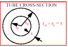
Input variables are system parameters that can be changed to improve the system performance such as beam dimensions, material properties, diameter, number of bolts, and so on. Input variables can be of different types with respect to their physical and/or numerical nature. Physically they can be dimensions, material properties, locations, etc. Numerically they can be continuous numbers, discrete, integer, real, strings. Optimization formulations are grouped as continuous, discrete or mixed continuous-discrete with respect to the numerical properties of the input variables. Selection of input variables may not be unique as seen in the example below. In this example, one can either pick ri and ro or ri and t as input variables.
Figure 1: Example for Input Variables Definition Input variables should be independent of each other. Also, for a larger search space and increased flexibility in the solution, we need to use as many as possible independent input variables but for computational affordability, we need to identify and only include the most important ones.
|
Objective functions are output responses that are required to be minimized (maximized). These output responses are functions of the input variables. Mass, stress, displacement, frequency and pressure drop are some examples of objective functions. Objective functions numerically can be grouped as linear and non-linear functions.
Optimization problems can be grouped as single or multi-objective optimization problems depending on how many objectives are considered. Multi-objective optimization (MOO) objective functions are formulated as:
such that When dealing with multiple objectives Usually the computational effort required to solve MOO problems are significantly more compared to single objective optimization problems. In cases where solving MOO problems are prohibitive, these problems have been converted to a single objective problem by summing all the objectives (Weighted Sum Method). When dealing with probabilistic variables, the objective function also has an associated distribution. When doing robust optimization, instead of the deterministic objective, the objective function is the value of the objective distribution at a specified value of the cumulative distribution function (CDF). A minimization problem might use the 95% value of the CDF (default value), and a maximization problem might use the 5% value of the CDF. For more information on probabilistic variables, refer to Uncertainty in Design.
|
Constraint functions are system requirements that need to be satisfied for the design to be acceptable such as requirements on displacement, frequency, pressure drop, cost, etc. These functions are also functions of the input variables.
|
When we put input variables, objectives and constraints together, we get the optimization formulation for a design problem as:
Objective |
min f(x) |
min cost ($) |
|
Constraints |
g(x) ≤ 0.0 |
h(x) = 0.0 |
|
σ < σallowable |
|
Design Space |
lower xi ≤ xi ≤ upper xi |
2.5 mm < thickness < 5.0 mm |
|
number of bolts ∈ (20, 22, 24, 26, 28, 30) |
Where:
| • | f(x) is the vector of system output responses that are used as objectives |
| • | g(x) and h(x) is the vector or system output responses that are used as inequality and equality constraints. |
| • | x is the vector of input variables |
Some of the results that would be reported after an optimization run include but not limited to:
|
The point or design that minimized (maximized) the objective function and at the same time satisfy all the constraints. |
||
|
Constraint that is not satisfied |
||
|
One that is satisfied exactly; equality constraints are active for feasible designs. |
||
|
One that satisfied but not on the bound. |
||
|
A point or a design that satisfies all the constraints. |
||
|
A design that violates one or more constraints. |
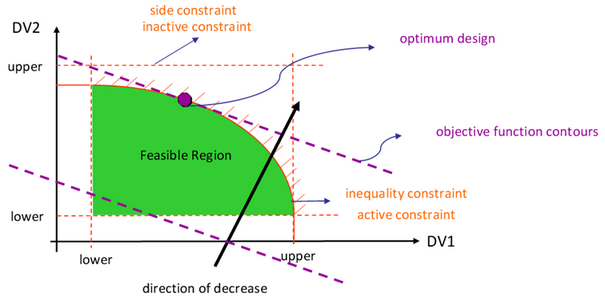
Figure 2: Design Space Definitions
In addition to minimization or maximization of objective function(s); three specific optimization problem formulations are also handled in HyperStudy:
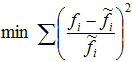
System Identification helps to move a set of output responses towards their target values. Examples for typical applications are experimental curve fitting or parameter fitting. The objective function is formulated as a least squares formula, as described below, where
|
Optimization problem formulation used to solve problems where the maximum (or minimum) of an output response is minimized (or maximized). The MinMax problem is formulated as follows:
These problems are solved using the Beta-method. In this method the problem is transformed into a regular optimization problem by introducing an additional input variable such that:
|
Optimization problems can also be categorized as deterministic or probabilistic, depending on the design requirements. Probabilistic problem formulations take into account the variability in the design and study the corresponding variability in the performances. This aspect is studied under reliability and robustness.