A new Python based lexicon for MotionSolve is provided in this release. Using this lexicon, one can now create Python applications that can:

For instance, you could: Perform a MotionSolve simulation and display live plots during the simulation with Matplotlib (a Python based plotting tool).

Along with the Python based lexicon, a new Python lexicon Reference Manual is also available.

Supported Entities

With this release, MotionSolve supports multi-iterative coupling (MIC) while co-simulating with AcuSolve. This enhancement allows MotionSolve to re-compute its system states on the fly when needed during co-simulation. This is helpful while trying to solve “tightly” coupled problems more accurately. With this enhancement, your co-simulation results are more accurate and the co-simulation is more robust.

You can use the MS_USERDLL_DIR environment variable to specify the location of your Python scripts (*.py, *.pyc) as well as your C++/FORTRAN user subroutines.

The environment variable MS_USERDLL_DIR can be set to a list of folder locations on your machine (separated by ;) where you want MotionSolve to search for your user subroutines (*.dll, *.so). This scenario is common when you don’t specify the absolute path of the user subroutine in your model or if the user subroutine is not in the same location as the solver input XML file.

A GUI option is available to specify geometric stiffness.

Selecting the highlighted option would include the relevant CMSMETH statement of the form CMSMETH, 1, CBG, , 15 into the FEM File.

“Include geometric stiffening” checkbox is now available in the Flex-body panel. This option will only be activated when the flex h3d contains the geometric stiff (GEOSTIFF) data that is saved while generating the flexible body during the CMS process.

Checking on this option will enable export of the geometric stiffness data into MotionSolve XML file.

The “Modes” dialog in the flex-body panel now contains an additional column to control export of geometric stiffness data for each mode.

Turning off geometric stiffness data for certain modes can significantly improve the solution time. However, you should be sure that the modes that are turned off have a minor influence on geometric stiffening effects.

The user subroutine build tool shipped with this release of MotionSolve now links with the msautoutils library on both Windows and Linux. You can now use access functions exported by the MotionAuto Utilities as well as the MotionSolve UserSub API. This substantially simplifies the effort on your part to create your own road or other Auto functionality based on the published set of capabilities.

The ISTAT return codes for the GTCMAT utility have been updated in MotionSolve.

Many enhancements have been added to Linear Analysis. These include:

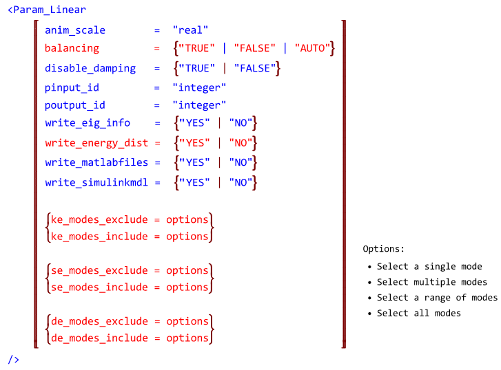
The updated statement is shown below with the 14.0 enhancements in red.

A new capability for “balancing” prior to eigenvalue analysis

For certain models, the eigenvalues calculated are sensitive to very minor changes in the state matrix used as input for the solution. This occurs when the eigenvector matrix is ill conditioned. MotionSolve detects an ill conditioned eigenvector matrix and “balances” the state matrix for a more robust eigenvalue solution.

Balancing refers to diagonally scaling the state matrix such that the row and column norms are numerically close to each other. You can control this behavior using the attribute “balancing” in the <Param_Linear> model or command statement.

Set “balancing” to “TRUE” to force MotionSolve to perform balancing on the state matrix and “FALSE” to disable balancing. The default for “balancing” is “AUTO” which lets the solver decide when balancing is required based on the condition number of the eigenvector matrix. Please note, that balancing is a very inexpensive operation.

Support for strain/dissipative energy calculations

For linear analyses, in addition to Kinetic Energy distribution, MotionSolve also calculates strain and dissipative energy for the following modeling elements:

The KE, strain and dissipative energy distribution is written to the log file, on the screen and the *_linz.mrf output file. To request MotionSolve to calculate these distributions, set the write_energy_dist attribute to “TRUE” in the <Param_Linear> model or command statement.

Mode selection for linear analysis output

You can now specify the modes for which MotionSolve writes the energy distribution on screen and to the log file. This is useful when the number of eigenmodes is large and you are interested only in a subset.

You may specify mode numbers to include or exclude, for each of the three distributions. Please see the documentation on <Param_Linear> for more details on how this is done.

With this release, the header for the PLT output files has been changed to allow the PLT file to be imported into FEMFAT for fatigue analysis. The old and new PLT format are described below:

Old format: The old format contains 4 columns for each request and the version number is 8.1.

New format: The new format contains 5 columns for each request and the version number is 9.1. The fifth column is added as per the specifications from FEMFAT. If this value is non-zero, then the next line is treated as a comment line.

Previously, MotionSolve did not solve models that have 0 DOF and time dependent loading. To solve such models you needed a workaround with “dummy” differential equations etc. With this release, MotionSolve has been enhanced to recognize 0 DOF models that have time dependent loading such that the simulation can continue. Such a scenario is useful when trying to determine joint reaction forces for models with 0 DOFs.

The definitions of the functions FX, FY, FZ, TX, TY and TZ have been made consistent with what is used in ADAMS. The table below lists the changes, using the FX function as an example:

MotionSolve now supports the adm statement GRAPHICS/… for displaying force vectors in the animation H3D. A sample statement is

GRAPHICS/10215001, FORCE, ETYPE=ALL, EM=10215001

The following ETYPE are now supported:

Previously, a model that had multiple SAVE/RELOAD statements and analyses with different output steps was not translated correctly to MotionSolve. An example of such a scenario is shown below:

RELOAD/SYSTEM, FILE=model.case5

SIM/STA, END=5.0, STEP=20

SIM/STA, END=6.0, STEP=5

SIM/STA, END=6.1, STEP=5

SIM/STA, END=6.5, STEP=4

SIM/STA, END=6.9, STEP=4

SIM/STA, END=7.0, STEP=5

This has been resolved within this release.