Model Description

Model location: <altair>\utility\mbd\nlfe\validationmanual\model6.mdl

This model consists of a 20 m length of wire attached between a fixed support at A and a collar at B. The wire has a mass per unit length of 0.2 kg/m. The collar can slide over a cylindrical frame. A horizontal force P of 20 N is applied on the collar.

The sag “h” and the span “L” of the cable is to be found.

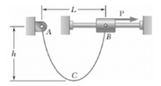
Figure 1: Problem description

Multi-Body Model

The cable is modeled using 20 NLFE cable elements. The fixed support, frame, and collar are modeled as rigid bodies.

The fixed support and frame are fixed-to-ground using fixed joints. The collar is connected to the frame using a translation joint. The cable is connected to the fixed support and collar using ball joints. A force of 20 N is applied to the collar via a STEP function as:

`Step (time, 0, 0, 5, 20) `

Even though this is a static equilibrium problem, the load is applied gradually and solved for a 10 second quasi-static simulation for the ease of solving.

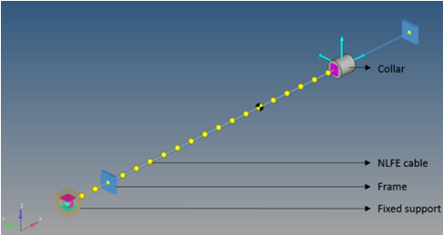
Figure 2: The cable problem modeled in MotionView

The theoretical solution is as follows.

Sag,   h = 4.09 m

Span, L = 17.69 m

This parameter can control the bending stiffness of the cable based on requirement in various cases.

Case 1

Consider the case of a single stranded cable, i.e., “Number of fibers” = 1

If the cable is very slender (for example, 1000 mm length and 0.1 mm diameter), then the bending stiffness is negligible. However, if the cable is less slender (for example, 1000 mm length and 10 mm diameter), the bending stiffness will become significant. In both situations MotionSolve automatically calculates the appropriate bending stiffness.

Case 2

Consider the case of a multi-stranded cable, for example, “Number of fibers” = X

For a cable that is less slender (for example, 1000 mm length and 10 mm diameter), the overall bending stiffness need not be significant – this is because the interactions between the fibers is a complex phenomenon that can make the bending stiffness negligible. The diameter in this case is calculated based on the cumulative area of all fibers.

Therefore, to get the actual or physical bending stiffness of the cable, the parameter “Number of fibers” can be tuned in MotionSolve. The bending stiffness of the cable element in MotionSolve decreases as you increase the “Number of fibers”.

In this particular problem, the calculations assume a theoretical cable with a bending stiffness of zero.

You can try to use the parameter “Number of fibers” in MotionSolve to see if you are able to get a closer correlation with the results produced assuming a theoretical cable. The number of fibers may need to be increased until the bending stiffness becomes negligible and saturated.

Numerical Results

The initial equilibrium position of the cable system at 0 seconds is shown below in Fig 3:

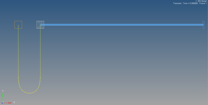
Figure 3: The initial equilibrium position of the cable system seen in HyperView animation.

The final equilibrium position of the cable system at the end of 10 seconds is shown below in Fig 4:

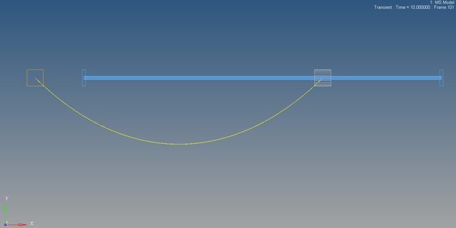
Figure 4: The final equilibrium position of the cable system seen in HyperView animation.

The Y position of Point_11 (the mid-point of cable) is plotted to find the sag “h”.

The X position of Point_21 (the end-point of cable) is plotted to find the span “L”.

“Number of fibers=1”

Figure 5 below depicts the sag “h” of the cable with parameter “Number of fibers=1”.

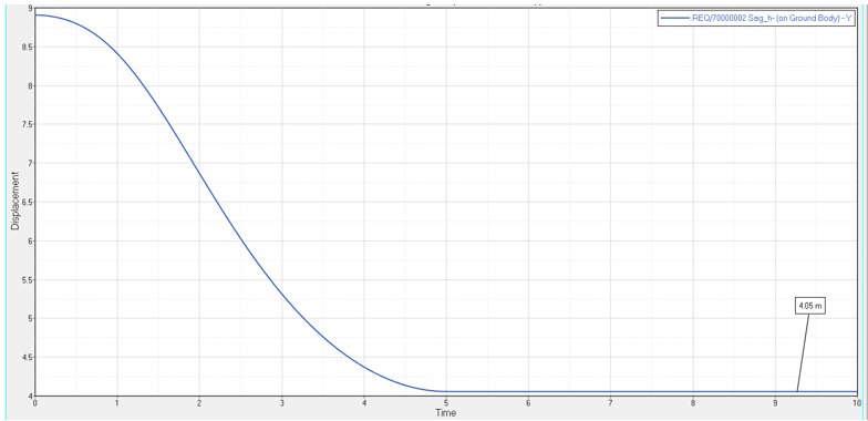
Figure 5: Plot showing sag “h” of the cable.

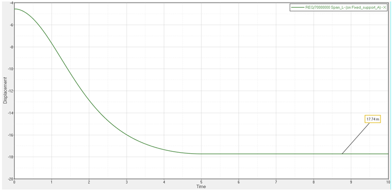
Figure 6: Plot showing span “L” of the cable.

Number of fibers=20”

Figure 7 below depicts the sag “h” of the cable with parameter “Number of fibers=20”.

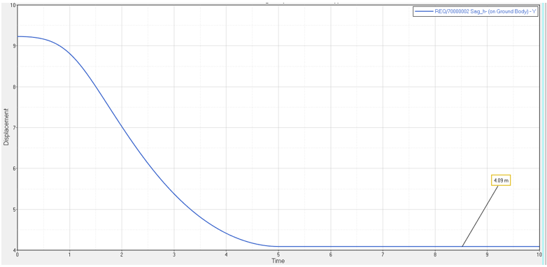
Figure 7: Plot showing sag “h” of the cable.

Figure 8 below depicts the span “L” of the cable with parameter “Number of fibers=20”.

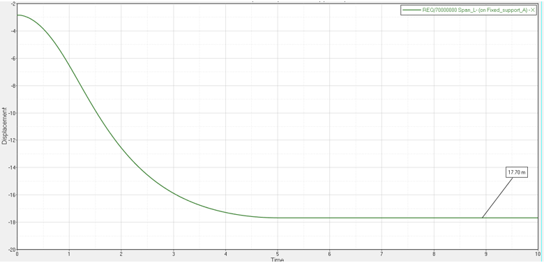
Figure 8: Plot showing span “L” of the cable.

Conclusion

The NLFE model shows close agreement to the theoretical results for this case. We see that by increasing the number of fibers, we can get closer to the theoretical results (that assumes zero bending stiffness).

The use of fibers is not only for the purpose of matching theoretical results. Any physical case of a multi-stranded cable with any bending stiffness can be modeled by tuning the parameter “Number of fibers”.