Command Element

Description

The DebugOutput command generates debugging output from MotionSolve.  These extra diagnostics are typically used to understand MotionSolve analysis failures, so that modeling issues may be fixed and simulation parameters may be changed to get past the failure(s).

Debug output falls into two categories:

The attributes below are used to identify and fix modeling issues.

Format

<DebugOutput

[ switch_on       = "TRUE" || "FALSE" ]

[ debug_anim      = "TRUE" || "FALSE" ]

[ screen_output   = "TRUE" || "FALSE" ]

/>

Attributes

switch_on

A logical flag that controls the generation of debugging information about the solver analysis steps, especially regarding the Newton-Raphson numerical method used by statics, quasi-statics and dynamics.  This messaging can be used to identify the modeling entities that cause the largest convergence error.  For a MotionSolve failure, look at the entities that are giving the integrator trouble right before the solver fails and investigate these first.  Generally, assuming that there is no modeling error, look for discontinuities in the model, and read the error messaging that MotionSolve reports.  This parameter can have values of “TRUE” or “FALSE”.

When not specified, switch_on defaults to “FALSE”.

Note: By default, the debug information is written only to the log file.  To change this, see screen_output.

debug_anim

A logical flag that controls the generation of animation frames at each iteration for debug purposes.  This animation is often helpful to determine how the models is being corrected (that is, repositioned) in Newton-Raphson and possibly give you clues on how to change the modeling or MotionSolve settings to find a converged solution.  It can have values of “TRUE” or “FALSE”.

When not specified, debug_anim defaults to “FALSE”.

The H3D file may be read into HyperView, and the results of the Newton-Raphson iteration may be visually examined.

See Comment 3 for more details.

screen_output

A logical flag that controls where the debug output information is written.  Choose between “TRUE” or “FALSE”.

When not specified, screen_output defaults to “FALSE”.

Comments

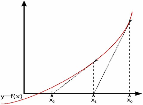
At the center of most of the output that comes from this command is a numerical method called  Newton-Raphson (N-R).  This method is used to solve a set of non-linear algebraic equations (NLAE’s).  This is a well-known method, often called “Newton’s method,” and you can find many sources that describe it.  This method finds the roots of the NLAE’s.  N-R is part of the solution process called the “corrector,” as it corrects an initial value to find a better solution to the NLAE’s.

N-R uses the partial derivatives of the non-linear algebraic equations with respect to the states of the system (the sensitivities) with the intent to progressively find a solution to the equations with less and less error.  The matrix of partial derivatives of these equations with respect to the states is called the “Jacobian”; thus, the Jacobian is essential to solving the N-R method.

In statics, quasi-statics, and dynamics, the equations of motion are converted into a set of non-linear algebraic equations (statics and quasi-statics, by virtue of setting all rates to zero; dynamics, by virtue of the integration method).  At each iteration, N-R tries to find a solution to the NLAE within the error tolerance.  If the solution is not within the error tolerance, N-R updates the states using the Jacobian and tries to find a better solution.  This process repeats until the error tolerance is met or the maximum number of iterations is exceeded.  See Param_Transient for more details).

In dynamics, if the maximum number of iterations is exceeded, the solver may try to take a smaller step size and attempt to solve the equations of motion again.  If, however, the integrator cannot cut the step size any more, the analysis will fail.  In statics, if the maximum number of iterations is exceeded, then the analysis fails, and you should examine the output from this command.

A very good way to understand N-R is to see it visually.  Below is a plot of a non-linear algebraic equation, y= f(x).  This image shows an equation with one variable, but this is generally applicable to equations with any number of variables.

Figure 1: Newton-Raphson method.

The equation can always be re-written such that f(x) = 0, and this is what N-R is solving to find the root, x*, such that f(x*) < error tolerance.

Here, the initial guess for the state x is x0.  If f(x0) > error tolerance (that is, it does not satisfy the error), then N-R computes the linear equation for f(x0) at x0, and uses this to compute a (hopefully) better solution at x1.  This new state, x1, is used to evaluate f(x1) and see if this is within the specified error tolerance.  You can see that for a non-linear equation like the example here, repeated iterations with N-R will become more and more accurate.  For some non-linear equations, this is not the case and N-R can actually diverge.

The slope of the linear equation (dotted line in the figure) used to update to the next state is effectively the Jacobian matrix – the partial derivatives of all equations with respect to the states in the system.  Updating the Jacobian at each iteration is generally a computationally expensive process, so sometimes this matrix is reused from prior iterations since the overall solution process is more efficient (see Param_Transient, dae_jacob_eval).

The debugging output you get with 'switch_on' and 'debug_anim' shows the N-R convergence information in table and graphical form, respectively.  When the solution does not converge, you should try to better understand what is going on in the model to either add, remove, or fix a modeling entity, changing the MotionSolve settings for the analysis.   Problems can arise if either the Jacobian does not have good information – which is the case for modeling entities that are discontinuous (non-smooth) or if the initial configuration of the system is far away from the final solution.

More details can be found in the subsequent comments.

switch_on potentially generates a lot of information and there is a significant performance penalty associated with its use.  Consequently, it should be used only when a model is being debugged.  See Comment 5 for more detail on the output that is generated.  This output may be used to further understand and diagnose the following scenarios:

This attribute is intended to aid visual debugging of a static analysis via the animation H3D in the HyperView post-procesor.  The attribute debug_anim writes out results at each iteration of the static simulation to the animation H3D and the output MRF file. This parameter should only be used while debugging a static simulation. If you set debug_anim to TRUE and run multiple simulations, MotionSolve quits with a warning message.

If you would like to debug a static analysis in a model that contains many analyses, you can use the <Save> and <Load_Model> command statements to isolate the static simulation that is of interest. Then you can use the debug_anim attribute to visually debug the convergence for static equilibrium.

Setting debug_anim to TRUE also potentially generates a lot of information and creates large H3D files.  There is significant performance penalty associated with its use.  Consequently, it should be used only when a model is debugged.

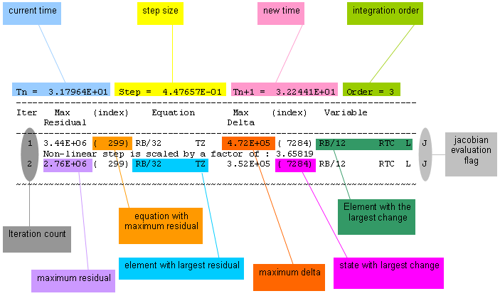
Figure 2 below shows the typical output in the log file when the attribute switch_on is set to TRUE.

Figure 2: Convergence history for a quasi-static analysis.

Figure 2 shows the details of the Newton-Raphson convergence history of the solution process for a step during a quasi-static analysis performed with a FIM_D.

At the top, the time step history is shown.  Referring to Figure 1 above, the information (shown in brick-red text) provided includes:

This is followed by the convergence history for the step.  Information about each iteration is contained in one line.  The data is column-ordered for easily identifying the information.  Once again, using Figure 2 as a reference, the data in each line includes:

When there is a modeling error, or a parameter value, such as bushing stiffness, is off scale, the debug data can be used to identify which modeling element may have the error.  Note that this is a symptom of the problem, not necessarily the entity that needs to be changed in the model.  For example, consider a rack and pinion-steering system with a coupler constraint that couples the rotational motion of the steering system to the translational motion of a rack.  If the coupler constraint is defined incorrectly, and tries to move the rack in a manner not intended, you may see the largest error reported in the rack body and/or constraints, rather than the problem in the coupler constraint itself.

The following table lists the short forms used to reference the commonly used modeling components.

In addition to the above, for the variable section (dark green in Figure 2), the element’s short form may be appended by one letter.  This letter indicates the kind of entity for which the maximum change is observed:

L - short name for Lambda, which refers to the constraint element terms.

A - short name for Acceleration, which refers to the acceleration terms (only for second order integrator).

V - short name for Velocity, which refers to the velocity terms.

D - short name for Displacement, which refers to the displacement terms.

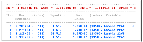
Figure 3 below depicts a sequence of iterations that is diverging.  This results in a “Corrector Failure.”

Figure 3: A sequence of diverging Newton-Raphson iterations.

In Figure 3, you can see that the error in the equations is not decreasing with each iteration; instead it is increasing.  The debug information (shown in blue) also indicates that equation 517, contained by modeling element G1-517, seems to have the most difficulty.  You can now go back to the input deck and try to understand why this could be so.

Conversely, if you see the error decreasing with each iteration, but the solver runs out of iterations (that is, exceeding the maximum number of iterations specified), then try to increase the maximum number of iterations to give the solver a chance to converge.

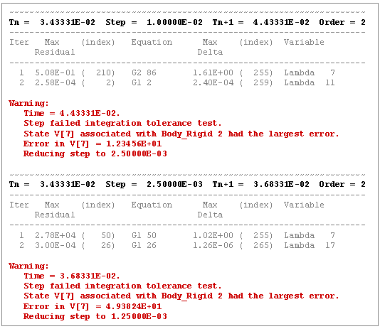
The corrector may be converging, but the integrator may be having difficulty satisfying the local error criterion. switch_on output may be used to understand why this is happening and help identify the root cause in the model.

Figure 4 below depicts a sequence of steps taken by DSTIFF using the Stabilized Index-1 formulation.  Assume that an integration error tolerance of 1.0E-3 was specified.

switch_on output at Time=3.43331E-02 seconds is shown for illustration purposes.

Figure 4: A sequence of failed integration steps.

The switch_on information in Figure 4 makes it quite clear that the corrector is not having any difficulty in converging to a solution.  However, the integrator is having difficulty satisfying the local error test.  The output also makes it clear that a system velocity associated in Rigid_Body 2 is showing the largest error.

One possible cause could be that a discontinuous motion is acting on Rigid_Body 2.  So, with this information, you can look at all Motion inputs on Rigid_Body 2.  A non-differentiable motion (a signal with “sharp corners”) is a likely cause, because the displacements seem to converge but the velocities are not.

switch_on output can also be used to determine whether the integrator is taking small steps and can help in identifying possible causes.  Small integration steps are being taken when the integrator is either having corrector convergence difficulties or large integration errors.  In either case, one can examine the output from switch_on and trace the difficulty back to a possible error or an unrealistic parameter (Mass, Stiffness, Damping, Discontinuity, and so on) in the model.

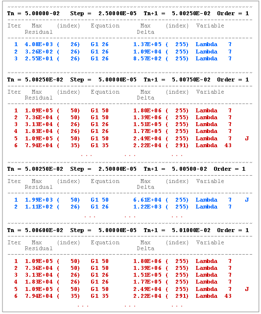
switch_on output can be used to detect and diagnose situations where the integrator is seemingly stuck at low integration orders.  The history of each step can be examined and the order noted.  If the order is low (for instance, Order=1 always) and the step size is small as shown in the example below, the situation is worth examining:

Figure 5: Simulation stuck at low order and step size.

In Figure 5 above, switch_on output for a series of steps with an Index-3 DAE formulation with an error tolerance = 1.0E-3 is shown.  You can note that the order of the simulation is seemingly stuck at one (1).  Furthermore, the simulation seems to be successful when the step size = 2.5E-05, but fails when a step of 5.0E-05 is attempted.  The failure is always because of non-convergence of the corrector.  You can also see that the Jacobian is evaluated automatically by DSTIFF.

A few strategies may be used to resolve the situation:

Example

<DebugOutput

switch_on   = "TRUE"

/>

Command Element

Description

The DEBUG command generates debugging output from MotionSolve. These extra diagnostics are typically used to understand MotionSolve's analysis failures, so that modeling issues may be fixed and simulation parameters may be changed to get past the failure(s).

Debug output falls into the following categories:

Declaration

def DEBUG(EPRINT=False, VERBOSE=False, ANIM=False):        

Attributes

EPRINT

A logical flag that controls the generation of debugging information about the solver analysis steps, especially regarding the Newton-Raphson numerical method used by statics, quasi-statics, and dynamics. This messaging can be used to identify the modeling entities that cause the largest convergence error. For a MotionSolve failure, look at the entities that are giving the integrator trouble right before the solver fails and investigate these first. Generally, assuming that there is no modeling error, look for discontinuities in the model, and read the error messaging that MotionSolve reports. This parameter can have values of TRUE or FALSE.

When not specified, EPRINT defaults to FALSE.

Note:  By default, the debug information is written only to the log file.  To change this, see VERBOSE.

VERBOSE

A logical flag that controls where the debug output information is written.  Choose between TRUE or FALSE.

When not specified, VERBOSE defaults to FALSE.

ANIM

A logical flag that controls the generation of animation frames at each iteration for debug purposes.  This animation is often helpful to determine how the models are being corrected (that is, repositioned) in Newton-Raphson and possibly give you clues on how to change the modeling or MotionSolve settings to find a converged solution.

It can have values of TRUE or FALSE.

When not specified, ANIM defaults to FALSE.

The H3D file may be read into HyperView, and the results of the Newton-Raphson iteration may be visually examined.

Comments

See DebugOutput

Example

The example below demonstrates how the DEBUG command is used.

DEBUG (EPRINT=TRUE)