Introduction
AcuSolve and RADIOSS are fully-integrated to perform a Direct Coupled Fluid-Structure Interaction (DC-FSI) Analysis based on a partitioned staggered approach. AcuSolve and RADIOSS are both time domain simulation codes that break the coupled simulation into a number of time steps. Because the governing equations of both AcuSolve and RADIOSS are nonlinear, sub-iterations are typically required within each time step. At each sub-iteration of FSI analysis, the fluid tractions in AcuSolve are converted into nodal forces which are then transferred to the structural interface mesh of RADIOSS. These forces are used to calculate the deformation of the structure using RADIOSS. Note that in addition to the load from the fluid flow tractions, additional structural loads can also be applied. The resulting deformed shape of structure is passed back to AcuSolve as the new fluid boundary. This FSI cycle is shown below in Figure 1.
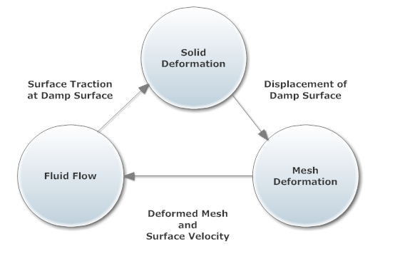
Figure 1: Direct-Coupled Fluid-Sstructure Interaction (DC-FSI) cycle
Target Applications
The DC-FSI capability aims at simulations of compliant structural response to fluid flow and its complex interrelationship. This capability is particularly suited for problems exhibiting nonlinear structural response. It may also be used for linear structural response; however, for linear structural response the P-FSI solution offered by AcuSolve may be more effective in solving the linearized structural response with the nonlinear flow solution. For further information on the P-FSI method, refer to the AcuSolve Command Reference Manual. Most RADIOSS features including nonlinear materials, nonlinear geometric effects, and contact are available for use. The interface domain can be modeled with solid, shell, and beam elements. Most of the features in AcuSolve can be used in DC-FSI simulations. These features may include, namely laminar or turbulent flow, heat transfer, a rich set of material options, free-surface and multi-species driven flows. The moving boundary problems are modeled using Arbitrary Lagrangian-Eulerian (ALE) and sliding mesh technologies. For further details, consult the AcuSolve Command Reference Manual.
Primary applications targeted by this capability include:
| • | Automotive: Hydraulically damped rubber mounts, door seals, shock absorbers, design of valves and rubber diaphragms and antilock braking systems |
| • | Oil/Gas: Long marine risers, moorings, free spans and drilling risers |
| • | Aerospace: Wing aero-elasticity, UAV and MAV |
| • | Wind turbine: Large deformation of blades |
| • | Consumer Goods: design and packaging |
DC-FSI using RADIOSS and AcuSolve
The following workflow is strongly recommended for solving DC-FSI problems:
| 1. | Develop RADIOSS structural model and an AcuSolve-only fluid model, and ensure that the uncoupled analyses run successfully. |
| 2. | Prepare the stand-alone models that include DC-FSI commands. |
| 3. | Run the coupled analysis. |
| 4. | Post-process the FSI solution. |
This workflow ensures that both the RADIOSS and the AcuSolve models are defined properly prior to performing a coupled simulation. RADIOSS and AcuSolve do not require that the analysis be run with a particular unit system, but both analyses need to use a consistent unit system. As a rule, all quantities exchanged between the two solvers will be in dimensional form, and the components of all vector quantities will be resolved in the inertial frame. For consistency, identical inertial frames must be selected for AcuSolve and RADIOSS.
RADIOSS Model
Preparing the RADIOSS model for DC-FSI involves three steps:
| • | Create input deck for RADIOSS |
| • | Identify the interface region and the solution quantities exchanged |
| • | Define the communication scheme |
The RADIOSS FSI input data that has the Engine keyword /IMPL/DYNA/FSI is shown below:
/IMPL/DYNA/FSI
ESET SSET PORT MINX MAXX TAG DATA MSG WAIT INIT
FTOL DTOL TTOL XTOL
Each of the data items are discussed below under their relevant topic.
The Damp Surfaces
The damp surface of the structural mesh must be specified in the RADIOSS FSI input data. The damp surface can either be specified by a group of elements or a surface. Note that the structural mesh on the damp surface does not have to match the interfacing fluid mesh. AcuSolve will internally project the CFD tractions from the fluid interface mesh onto a non-matching damp surface structural mesh. The mapping of nodal forces is also supported for structural beam elements. For example, a rod, pipe or blade can be modeled with simple beam elements in the structural mesh. The corresponding fluid mesh will contain the actual three-dimensional geometry of these beam elements.
If the damp surface is specified by a group of elements (ESET), use the /GRBEAM/BEAM/, /GRSHEL/SHEL/, or /GRSH3N/SH3N/ data for beam, 4-node, and 3-node shell elements, respectively. It is possible to specify the damp surface of a solid by coating it with shell elements and then assigning these elements zero material properties using the /MAT/LAW0 data. If the damp surface consists of beam elements, then these must be specified using the beam element group data. The ID of the element group is the first item of the /IMPL/DYNA/FSI data.
The damp surface (SSET) can also be specified by the RADIOSS /SURF data. The /SURF data has many options that can be used to specify a surface. The surface can be either the surface of a shell structure or the surface of a solid mesh. The surface ID is the second item of the /IMPL/DYNA/FSI data. Note that beam elements cannot be specified using the /SURF data.
Note that the damp surface can be defined by a combination of an element group and a surface.
The matching fluid surface is specified in the AcuSolve data using the EXTERNAL_CODE_SURFACE command.
In some cases a portion of the structural damp surface must be “tagged” so that AcuSolve can associate it with the AcuSolve boundary surface. This is done by specifying the RADIOSS part ID as the external_code_tags parameter in the EXTERNAL_CODE_SURFACE data.
Example:
EXTERNAL_CODE_SURFACE( "Drill" ) {
...
external_code_tags = {"10"}
...
}
Data is used to specify that this surface corresponds to the RADIOSS part with ID 10. Note that each individual surface must consist of elements with the same part ID, and each separate surface must consist of elements with separate part ID’s. In order to apply a tag, the surface of a solid structure, the solid must be coated with shell elements and the property ID of these shell elements used as the surface tag. To specify the use of surface tags, set item 10 of the /IMPL/DYNA/FSI data (TAG) to 1.
AcuSolve Model
This section provides an overview for preparing the AcuSolve model for DC-FSI. For detailed information on the commands, refer to the AcuSolve Command Reference Manual. The three steps to prepare the AcuSolve model are:
| 1. | Set the analysis parameters to include an external field. |
| 2. | Define the solution strategy. |
| 3. | Define the external surface definition. |
Setting Analysis Parameters to Include an External Field
Use the EQUATION command to specify the solution fields available or the system of equation that are present in the problem. To include a field that is computed with an external solver, for RADIOSS, set the external_code parameter to 'ON'.
For example, when conducting a fluid-structure analysis in which AcuSolve computes the flow and RADIOSS computes displacements, turn ON the external_code parameter and allow for arbitrary mesh movement by setting the mesh parameter to arbitrary_lagrange_eulerian.
EQUATION {
| mesh | = arbitrary_lagrange_eulerian |
}
Defining the Solution Strategy
In conjunction to the EQUATION command, which specifies the existence of solution fields in the problem, you must use TIME_SEQUENCE and STAGGER commands to define time stepping and staggering strategy. The preferred method is to use the AUTO_SOLUTION_STRATEGY command to have AcuSolve generate the solution strategy commands. In order to highlight the solution strategy commands, highlight the TIME_SEQUENCE and STAGGER commands.
The TIME_SEQUENCE command specifies the time stepping and staggering strategy. In the following example, the external field is solved first for structural displacements, which is then followed by the mesh displacement (ALE) in which the fluid elements are adjusted. Then the flow and turbulence equations are solved.
TIME_SEQUENCE {
min_time_steps = 1
max_time_steps = 15
:
min_stagger_iterations = 1
max_stagger_iterations = 20
staggers = { "external_code",
"mesh_displacement",
"flow",
"turbulence" }
}
For each of the fields being solved (each stagger defined in the TIME_SEQUENCE command), one needs to define the nonlinear iteration and linear solver parameters. This is done using the STAGGER command. For example, the STAGGER commands are shown for external_code, mesh_displacement, and flow equations.
STAGGER ( "external_code” ) {
equation = external_code
min_stagger_iterations = 1
max_stagger_iterations = 10
}
STAGGER( "mesh_displacement" ) {
equation = mesh_displacement
min_stagger_iterations = 1
max_stagger_iterations = 5
convergence_tolerance = 0.1
linear_solver = conjugate_gradient
min_linear_solver_iterations = 10
max_linear_solver_iterations = 1000
linear_solver_tolerance = 0.001
projection = off
}
STAGGER( "flow" ) {
equation = flow
min_stagger_iterations = 1
max_stagger_iterations = 2
convergence_tolerance = 0.1
lhs_update_frequency = 1
linear_solver = gmres
linear_solver_tolerance = 0.1
}
Defining the Fluid-Structure Interface
Use the EXTERNAL_CODE_SURFACE command to define the interface between the fluid and structure. The command specifies the surface topology, as well as the interface proprieties.
In the following example, the interface surface topology is read from the file wall.ebc located in the MESH.DIR directory and consists of 3-node triangles. The velocity_type, temperature_type, and mesh_displacement_type define the interface properties (boundary conditions) and are discussed below.
EXTERNAL_CODE_SURFACE( "wall" ) {
| surfaces | = Read( "MESH.DIR/wall.ebc" ) |
| shape | = "three_node_triangle" |
| mesh_displacement_type | = tied |
}
The interface properties or boundary conditions are specified through the mesh_displacement_type, velocity_type, and temperature_type parameters. The mesh_displacement parameter defines whether the fluid mesh is tied to the solid mesh or allowed to slip against the solid mesh surface. Set the mesh_displacement_type=tied to tie the fluid mesh to the solid mesh, or mesh_displacement_type=slip to allow the fluid mesh to slide against the solid surface, which acts as a guide surface.
The velocity_type specifies how the fluid velocity behaves in relation to the structural mesh velocity. Set velocity_type=wall to tie the fluid velocity to the mesh velocity, or set velocity_type=slip for the normal component of the fluid velocity to be tied to the solid mesh velocity.
There are four possible interface combinations based on the settings of the mesh_displacement and velocity_type parameters. These are summarized in Table 1.
Fluid-Solid Interface Conditions
|
Mesh Displacement
|
Tied
|
Slip
|
Velocity Type
|
Wall
|
|


|
Slip
|
|
|
Table 1: Direct-Coupled Fluid-Structure Interaction Boundary Conditions
When the fluid is allowed to slide along the solid mesh, neighborhood searches between the fluid and solid meshes are continuous performed. The gap_factor parameter specifies a non-dimensional (with respect to the length of the element face) maximum allowable gap and the gap parameter specified a dimensional maximum gap distance between each quadrature point of the AcuSolve surface to the closest surface given by RADIOSS to check for gaps. If the distance is greater than the gap, the computation stops with an error message.
Communication between AcuSolve and RADIOSS
RADIOSS and AcuSolve can be run on heterogeneous and remote platforms which are located on the same network domain. The communication between RADIOSS and AcuSolve is via sockets. To start a co-simulation between RADIOSS and AcuSolve, one of the analysis software needs to initiate the communication process, while the other analysis software needs to connect to the initiated communication process.
In RADIOSS the socket port number (PORT) is specified by the third item of the /IMPL/DYNA/FSI data. The default port number is 10000. This same port number must be specified in the EXTERNAL_CODE data in the AcuSolve.inp file. If the machine that RADIOSS is running on is named unix_mach, then the EXTERNAL_CODE will look like:
EXTERNAL_CODE {
}
AcuSolve and RADIOSS are started independently. AcuSolve will wait for RADIOSS to initiate the socket connection. The time that AcuSolve will wait is determined by the WAIT parameter of the /IMPL/DYNA/FSI data. The default value is 3600 seconds.
Before the start of time step loop, basic information about the interface must be exchanged between the two codes. First, a number of parameters controlling the interface strategy must be set for both codes. Second, the physical parameters of the interface must be defined. Typically, both AcuSolve and RADIOSS start at the same time step; however, if there is a desire to have AcuSolve start first (to allow for the flow to develop), the INIT data of the /IMPL/DYNA/FSI data can be set to the initial AcuSolve time step at which the coupled analysis will start.
Time Steps and Data Exchanges
Both RADIOSS and AcuSolve need to use the same time step size and the total number of time steps should be the same. Also, the size of the time step needs to remain constant in both RADIOSS and AcuSolve. For example, for 1000 time steps of 0.001 seconds the AcuSolve and RADIOSS data are:
AUTO_SOLUTION_STRATEGY {
| initial_time_increment | = 0.001 |
| min_stagger_iterations | = 1 |
| max_stagger_iterations | = 20 |
}
and
/RUN/wing/1
1.0
/IMPL/DTINI
0.001
/IMPL/DT/2
12 0.0 120 1.0 1.0
For the RADIOSS input data /IMPL/DT/2, items 4 and 5 specify the time step scale factors. These need to be set to 1.0 in order to keep the RADIOSS time step constant.
At each time step, the forces and displacements are exchanged between RADIOSS and AcuSolve until they converge to a certain tolerance. Once convergence is achieved, the analysis continues on to the next time step. These exchanges are called "staggers" in AcuSolve. The minimum number of staggers (exchanges) should be set to 1 in both sets of input data. This is specified by the min_stagger_iterations parameter in the AcuSolve AUTO_SOLUTION_STRATEGY data and the MINX data in the RADIOSS /IMPL/DYNA/FSI data.
The maximum number of exchanges can be controlled by a combination of force and displacement convergence criteria and a hard limit on the maximum number of exchanges. The maximum number of exchanges is set by the max_stagger_iterations parameter in the AcuSolve AUTO_SOLUTION_STRATEGY data and the MAXX data in the RADIOSS /IMPL/DYNA/FSI data.
Force and displacement convergence tolerances are used to reduce the number of exchanges to the number needed to receive stable and accurate results. This can dramatically reduce run times while guaranteeing accurate results. The force and displacement tolerances are specified by the FTOL and DTOL data in the RADIOSS /IMPL/DYNA/FSI data. These are tolerances on the L2 norms of the force and displacement vectors. If these tolerances are set high, the solution time will be reduced, but solution accuracy may also be reduced.
Typically, only forces and displacements need to be exchanged. In special cases, such as a spinning beam, you can request that moments and rotations are also exchanged. This is done by setting the DATA parameter to 2 of the RADIOSS /IMPL/DYNA/FSI data.
Data Exchange Verification
In order to verify that the correct data is being exchanged between RADIOSS and AcuSolve, the MSG parameter can be set to a non-zero value of the RADIOSS /IMPL/DYNA/FSI data. The higher the value, the greater the amount of information that is written to the RADIOSS .out file for verification. This data includes the data communication control parameters, as well as the actual values of the forces and moments being exchanged.
Examples
Typically, you only need to define the damp surface to run Fluid-Structure Interaction Analysis with RADIOSS and AcuSolve. If the damp surface has a surface ID of 10, the input data would be:
/IMPL/DYNA/FSI
0 10 0 0 0 0 0 0 0 0
0 0 0 0
In this case, all of the other FSI parameters are set to their default values. Note that in RADIOSS, 0 means the default value and not explicitly zero (unless the default value is actually zero).
In order to reduce run times, you could set an upper bound on the number of exchanges, as well as setting higher values for the force and displacement convergence tolerances. For example, you could set the maximum number of exchanges to 5 and the force and displacement convergence tolerances to 0.01 and 0.005 respectively with the FSI data:
/IMPL/DYNA/FSI
0 10 0 0 5 0 0 0 0 0
0.01 0.005 0 0
In the case of a beam problem with tagged elements and the exchange of moments and rotations, the input data would be:
/IMPL/DYNA/FSI
20 0 0 0 0 1 1 0 0 0
0 0 0 0
Where, 20 is the element set that contains all the beam elements. The beam element tags are based on the beam property ID’s.
Setting up the RADIOSS Structural FSI Data
The structural analysis type is implicit dynamics and is solved using the General Newmark method, so the RADIOSS Engine Keyword is:
/IMPL/DYNA/2
Suggested RADIOSS time step convergence criteria are 0.001 for energy and force and 0.01 for displacement, as set on the Implicit Nonlinear Solution Control data:
/IMPL/NONLIN/1
123 0.001 0.001 0.01
Since the time step must remain constant, the Time Step Control method must allow for many time iterations without changing the time step and the scale factors on the time step must be 1.0. The Time Step Control method 2 data should be:
/IMPL/DT/2
12 0.0 120 1.0 1.0
Also, the number of allowable divergence iterations must be increased so that the time step is not adjusted. This is done by setting the Divergence Criterion to 5 with:
/IMPL/DIVERG/5
Finally, to write the applied loads from the fluid tractions and the resulting displacements to the RADIOSS results animation files, use:
/ANIM/VECT/FEXT
/ANIM/VECT/DISP
Locations of the Models
The RADIOSS and AcuSolve models must be co-located. In other words, fluid boundary mesh and the corresponding structural damp surface mesh match each other as physical boundary. The gap between these meshes should be small. To verify the conformity of exchange surfaces in AcuSolve, consult the .Log file for the structural mesh information, as shown below. Verify the number of damp surface elements and the minimum and maximum coordinates of the damp surface, as well as for matching bounding box and areas to help identify position, size and orientation mis-match:
acuSolve: No. external code nodes = 15050
acuSolve: No. external code tri3s = 0
acuSolve: No. external code quad4s = 15000
acuSolve: Min/Max x-coord = -3.812500e-02 3.812500e-02
acuSolve: Min/Max y-coord = -3.805000e-02 3.805000e-02
acuSolve: Min/Max z-coord = 0.000000e+00 3.812500e+00
acuSolve: Total surface area = 9.126732e-01
acuSolve: No. fluid damp surfaces = 5637
acuSolve: Min/Max x-coord = -3.812499e-02 3.812500e-02
acuSolve: Min/Max y-coord = -3.812494e-02 3.812498e-02
acuSolve: Min/Max z-coord = 0.000000e+00 3.812500e+00
acuSolve: Total fluid surface area = 9.128247e-01
At each time step the damp surface deforms, due to the fluid flow load. At the same time, the fluid mesh is moved to match the new damp surface. The average and maximum gap between the meshes is shown for each time step as:
acuSolve: Ave distance = 2.842759e-05
acuSolve: Max distance = 1.182390e-04
The gap should remain small for a valid solution.
Post-processing the Coupled Simulation
There are a couple of options to post-process the coupled simulation:
| • | Post-process the structural solution and interface response using HyperView and the fluid solution and interface response using a post-processor compatible with AcuSolve, such as HyperView. |
| • | Use a third-party post-processing software to post-process the combined structural and fluid solution. |
Scaling of Quantities
You may apply a multiplier function in AcuSolve to the forces and/or moments imported from RADIOSS. Scaling fields may be useful when starting a fluid-structure interaction simulation with high inertial effects. Specify a multiplier function on the EXTERNAL_CODE command.
MULTIPLIER_FUNCTION("ramp" ) {
| curve_fit_values | = { 1, 0.0 ; 10 , 1 } |
| curve_fit_variable | = time_step |
}
EXTERNAL_CODE {
…
| multiplier_function | = "ramp" |
…
}
Parallel Execution of the Solvers
AcuSolve and RADIOSS may be run in parallel on distributed memory clusters.
Platform Support
AcuSolveTM runs on Windows (64-bit), Linux (64-bit) and many versions of UNIX.
Limitations
| • | If the damp surface contains beam elements, no other elements can be used to define the damp surface. In other words, beam elements cannot be mixed with other elements to define the damp surface. |
| • | Quadratic and modified tetrahedral elements are not supported |
| • | There must be a constant locked time step increment between two solvers |
| • | Thermal analysis is not supported at this time |


