|
»Click here to display Table of Contents«
|

Modeling Contacts |

|

|

|

|
|
Modeling Contacts |
|
|
|

|
|
»Click here to display Table of Contents«
|
Modeling Contacts |
|
|
|
|
|
Modeling Contacts |
|
|
|
|
MotionSolve provides a very sophisticated contact modeling capability that can handle complex contact scenarios between rigid bodies. To simulate rigid body contact in your model, you need to:
| • | Identify geometries two bodies that can come into contact with each other. MotionSolve allows you several options to define these geometries. |
| • | Specify contact material properties such as stiffness, damping, coefficient of restitution, friction etc. MotionSolve monitors the proximity of the specified geometries to each other. When any contact between the two sets of geometry occurs, a force based on the defined physical properties is generated. This represents the contact force. Both normal as well as frictional forces can be modeled. When the bodies separate, the force becomes zero. |
There are three key features to the contact capability in MotionSolve:
| • | Modeling the geometry of the bodies that are in contact. |
| • | Detecting contact. |
| • | Applying the contact force. |
There are several options for defining the geometry of the bodies in contact. For simple shapes, you may use MotionSolve primitive graphics, such as cylinder, box, plane, frustum, and ellipsoid. These graphics are tessellated automatically by MotionSolve using triangular elements. More complex geometries may be defined using a CAD package and imported into MotionView after translating them into the H3D format. You can perform this translation by going to the MotionView Tools menu and selecting Create graphics from CAD or Mesh…. The H3D file contains tessellated geometry that MotionSolve understands. Alternatively, you can define the geometry as a Parasolid graphic by directly importing the graphic in the Graphics panel. On export to MotionSolve, the Parasolid graphic is tessellated using triangular elements.
MotionSolve also lets you simulate contact that occurs along a curve between two geometries. For this case, you may define two curves, one on each rigid body involved, and use a specialized 2D curve-to-curve contact algorithm that may provide more accurate results and simulate contact faster than the 3D rigid body contact. It is assumed that the contact occurs only in the plane of the two curves that are defined. In other words, no out of plane contact forces are expected.
The quality and accuracy of the contact force calculated by MotionSolve depends greatly on the quality of the mesh/curve for the graphics that are used in the contact simulation. For tips and best practices on meshing graphics for contact in MotionSolve, please see Best Practices for Modeling 3D Contacts.
When the onset of a collision is detected, the collision detection algorithm returns the set of interfering triangles. From those, MotionSolve computes the following:
| • | The point of contact and surface normal vector. The penetration depth is determined from these quantities. |
| • | The magnitude and direction of the normal and friction forces. |
The choice of the solver step size becomes important while trying to accurately capture the onset of first contact. If the step size is not small enough to detect the contact event, large penetrations may occur that result in large contact forces. To avoid these situations, MotionSolve provides a sensor that monitors the onset of contact and automatically changes the solver step size to accurately determine the first contact event. This leads to more realistic contact forces without having to reduce the step size for the entire simulation. For more information on how to use this, please refer to the Sensor: Event modeling element.
Once the point of contact, penetration depth and surface normal vector are known, the normal and friction force magnitudes are computed using one of the following models:
| • | Poisson or penalty based model |
| • | Impact based model |
| • | Volume model |
| • | User defined model |
In all these models, the normal force is calculated based on “stiffness” and “damping” parameters. The table below lists the parameters that are used to calculate the normal contact force for each model.
|
Poisson model |
Impact model |
Volume model |
User defined |
Stiffness |
Penalty |
Stiffness, exponent |
Elastic modulus, layer depth, exponent |
User defined |
Damping |
Coefficient of restitution |
Damping coefficient |
Damping coefficient |
User defined |
If neither of these normal force models are suitable to the problem at hand, then a user written subroutine, CNFSUB, can be used to implement a custom normal force model.
| • | Static and dynamic Coulomb model |
| • | Dynamic only Coulomb model |
| • | User defined model |
The friction force is calculated as:
![]()
where
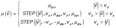
is the coefficient of friction for the static and dynamic Coulomb model and
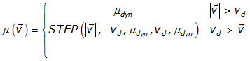
is the coefficient of friction for the dynamic only Coulomb model.
In the above equations:
| • |
| • |
| • |
| • |
| • |
| • |
| • |
For more information on these parameters, please refer to Force: Contact model element.
If such a friction force model is not suitable to the problem at hand, then a user written subroutine, CFFSUB, can be used to implement a custom friction force model.