Model Element

Description

Motion_Joint defines a motion input at a degree-of-freedom in a joint.  This input is allowed only on three types of joints:

Translational motions may be defined on Translational and Cylindrical joints.  Rotational motions may be defined on Revolute and Cylindrical joints.

You define an expression for the motion characteristics.  The expression may be used to define displacement, velocity, or acceleration.  The expression is usually a function of time.  See Comment 8 if you want to make the motion expression dependent on system states.

A translational motion is defined in one of the following ways:

A rotational motion may be defined in one of the ways listed below:

In the above, I is the i_marker_id of the joint and J to the j_marker_id. The software defines the state dependent term in the equations and you define the expression, the type of motion, and the joint on which the input is to be provided.

For a translational motion, the z-axis of j_marker_id defines the direction of positive motion.  The origin of i_marker_id moves along this line.  At zero displacement, the origins of the two markers are coincident.

For a rotational motion, i_marker_id rotates about the common z-axis.  A positive motion results in counter clockwise rotation.

A reaction force is associated with each Motion_Joint. This reaction force tells the system the force or torque that is needed to apply the requested motion.

When the expression is a function of time, energy is either added to or removed from the system.  Motion inputs may be considered as linear or rotational motors with infinite force or torque capacity.

The expression that you supply may be specified using either a MotionSolve expression or a user defined subroutine.

Format

<Motion_Joint

      id            = "integer"

    [ label         = "string" ]

      joint_id      = "integer"

      motion_type   = { "R" | "T" }

  {    

      val_type      = "D"

      val_type      = "V"

      ic_disp       = "real"

      val_type      = "A"

      ic_disp       = "real"

      ic_vel        = "real"

  }

  {

      type          = "EXPRESSION"

      expr          = "motionsolve_expression" >

      | type        = "USERSUB"

      usrsub_dll_name         = "valid_path_name"

      usrsub_param_string     = "USER( [[par_1 [, ...][,par_n]] )"

      usrsub_fnc_name         = "custome_fnc_name" >

      | type = "USERSUB"

        script_name         = valid_path_name

        interpreter         = "PYTHON" | "MATLAB"

        usrsub_param_string = "USER( [[par_1 [, ...][,par_n]] )"

        usrsub_fnc_name     = "custom_fnc_name" >

  }

</Motion_Joint>        

Attributes

id

Element identification number (integer>0).  This number is unique among all Motion_Joint elements.

label

The name of the Motion_Joint element.

joint_id          

Specifies the ID of the joint at which the motion input is applied.

motion_type        

Specifies the type of motion that is to be applied.  Motion types may be translational ("T") or rotational ("R"). Specify either "T" or "R". Note that motions on translation joints are always of type "T". Motions on revolute joints are always of type "R". Motions on cylindrical joints may be of either type, but not both.

val_type

Specifies whether the motion applies a displacement input (D), a velocity input (V), or an acceleration input (A). You must select one value from "D", "V", or "A".

ic_disp

Specifies the displacement initial condition that is required when val_type = "V" or val_type = "A".

ic_vel

Specifies the velocity initial condition that is required when val_type = "A".

type

Select either "EXPRESSION" or "USERSUB". Specifies how the motion is defined.  The EXPRESSION option specifies that the motion value is a MotionSolve expression that can be evaluated at run-time.  The USERSUB option indicates that the value of the motion value is specified in a user defined subroutine.  The parameters
"usrsub_param_string" and "usrsub_dll_name" are used to provide more information about the user defined subroutine.

expr

Defines an expression that defines the motion value. Use this parameter only when type = EXPRESSION. Any valid run-time MotionSolve expression can be provided as input.

usrsub_dll_name

Specifies the path and name of the DLL or shared library containing the user subroutine.  MotionSolve uses this information to load the user subroutine MOTSUB in the DLL at run time.

usrsub_param_string

The list of parameters that are passed from the data file to the user defined MOTSUB. Use this keyword only when type = USERSUB is selected.

usrsub_fnc_name

Specifies an alternative name for the user subroutine MOTSUB.

script_name

Specifies the path and name of the user written script that contains the routine specified by usrsub_fnc_name.

interpreter

Specifies the interpreted language that the user script is written in. Valid choices are MATLAB or PYTHON.

Comments

However, if VSTIFF, MSTIFF or ABAM are used, then the motions may only be functions of time.  To define the motions as a function of state, you must apply a time lag to the system data you are requesting and then smooth it as discussed below.

EXPR(Tk+1) = VR(100,200) evaluated at Tk,

Tk+1- Tk is the sampling period for the system.

Note that EXPR(Tk+1) is constant.  However it changes whenever the velocity VR() is sampled.  This implementation is not adequate because the sampled values are not continuous.  You must fit a curve through the previously sampled values and extrapolate the curve to provide a smooth value.  This is shown symbolically  below:

EXPR(Tk+1) = CUBIC(VR(100,200)|Tk, VR(100,200)|Tk-1, VR(100,200)|Tk-2)

Example

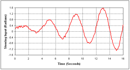
The first example shows how experimental data may be fed into the system as motion input.

Automotive vehicle handling simulations are often performed using semi-analytical simulation techniques.  A vehicle to be tested is instrumented with sensors to measure the steering wheel angle while it is being driven.  The vehicle is driven on the proving grounds.  The driver may perform a variety of maneuvers simulating real-life steering situations.  This data is collected as a function of time.

The experimental data is "cleaned" to remove noise and high frequency content.  Next, a vehicle model suitable for vehicle handling studies is created in MotionSolve.  The experimental data is modeled as a SPLINE in MotionSolve and it is provided as steering input to the analytical model of the vehicle.  During the simulation vehicle behavior necessary for evaluating handling are collected.

The steering input, after being "cleaned", might look as shown in Figure 1:

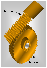
Experimentally measured steering input

The Motion_Joint for the steering input would like this:

<Motion_Joint

    id                  = "1"

    joint_id            = "301"

    motion_type         = "R"

    val_type            = "D"

    type                = "EXPRESSION"

    expr                = "CUBSPL(Time, 0, 301001)" >

</Motion_Marker>

The second example demonstrates how you may specify the motion of a worm and wheel mechanism using a Motion_Joint.  The image below illustrates the mechanism.

A worm wheel mechanism

The worm gear is driven by a motor at a constant rate of 200 revolutions per second.  Due to the gearing ratio, the wheel turns slowly relatively to the worm.  This is a speed reduction system ideally forming part of a drive or lifting device. Constraint_Joint 101 defines a revolute joint between the worm gear shaft and the housing.  A Motion_Joint on this revolute joint simulates the motor.  The motion definition would look as follows:

<Motion_Joint

    id                  = "2"

    joint_id            = "101"

    motion_type         = "R"

    val_type            = "D"

    type                = "EXPRESSION"

    expr                = "200*2*PI*Time" >

</Motion_Joint>

Model Element

Description

MOTION defines a motion input at a degree-of-freedom in a joint.  This input is allowed only on three types of joints:

Translational motions may be defined on Translational and Cylindrical joints.  Rotational motions may be defined on Revolute and Cylindrical joints.

You define an expression for the motion characteristics.  The expression may be used to define displacement, velocity, or acceleration.  The expression is usually a function of time.  However you may also make the motion expression dependent on system states.

A translational motion is defined in one of the following ways:

A rotational motion may be defined in one of the ways listed below:

In the above example, I refers to the i_marker_id of the joint and J to the j_marker_id.  The software defines the state dependent term in the equations and you define the expression, the type of motion, and the joint on which the input is to be provided.

For a translational motion, the z-axis of j_marker_id defines the direction of positive motion.  The origin of i_marker_id moves along this line.  At zero displacement, the origins of the two markers are coincident.

For a rotational motion, i_marker_id rotates about the common z-axis.  A positive motion results in counter clockwise rotation.

A reaction force is associated with each motion.  This reaction force tells the system the force or torque that is needed to apply the requested motion.

When the expression is a function of time, energy is either added to or removed from the system.  Motion inputs may be considered as linear or rotational motors with infinite force or torque capacity.

The expression that you supply may be specified using either a MotionSolve expression or a user defined subroutine.

Instead of defining motion on a joint, you may simply specify motion between two markers of two different parts.

The motion input may be translational or rotational.  You define an expression for the motion characteristics.  The expression may be used to define a displacement, velocity, or acceleration input.  The expression is usually a function of time but can also be made dependent on system states.

Translational motions may be defined in one of the ways listed below.

The functions DX(), DY(), and DZ() represent the x-, y- and z-components, respectively, of the translational displacement vector of the I marker, relative to the J marker, as measured in the coordinate system of the J marker.

The functions VX(), VY(), and VZ() represent the x-, y- and z-components, respectively, of the translational velocity vector of the I marker relative to the J marker, as measured in the coordinate system of the J marker. The time derivative is taken in the reference frame of the J ,marker.

The functions ACCX(), ACCY(), and ACCZ() represent the x-, y- and z-components, respectively, of the translational acceleration vector of the I marker relative to the J marker as measured in the coordinate system of the J Reference_Marker.  All time derivatives are taken in the reference frame of the J marker.

Rotational motions may be defined in one of the ways listed below.

B1(I,J), B2(I,J), and B3(I,J) represent the first, second, and third angles of the Body 1-2-3 Euler angle sequence that orients the I Reference_Marker with respect to the J marker.

Declaration

def MOTION(ID, LABEL="", JOINT=0, JTYPE="", I=0, J=0, DIRECTION="", DTYPE="", ICDISP=0.0, ICVEL=0.0, FUNCTION="", ROUTINE="", INTERPRETER="", SCRIPT=""):

Attributes

id

Element identification number (integer>0).  This number is unique among all the MOTION elements.  It uniquely identifies the modeling element.

LABEL

The name of the MOTION element.

JOINT

Specifies the ID of the joint at which the motion input is applied.

JTYPE

Specifies the type of motion that is to be applied.  Specify either "TRANSLATION" or "ROTATION".  Note that motions on translation joints are always of type "TRANSLATION".  Motions on revolute joints are always of type "ROTATION".  Motions on cylindrical joints may be of either type, but not both.

I

Specifies the marker ID at which the motion input is applied.

J

Specifies the marker ID from which the motion input is applied.

DIRECTION

Specifies the direction of the input.  Select one from "X", "Y", "Z", "B1", "B2", and"B3".

"X", "Y", and "Z" specify the direction for the translational motion.

"B1", "B2", "B3" specify the direction for the rotational motion.

DTYPE

Specifies whether the motion applies a displacement input, a velocity input, or an acceleration input.  You must select one value from "DISPLACEMENT", "VELOCITY",or "ACCELERATION".

ICDISP

Specifies the displacement initial condition that is required when DTYPE = "VELOCITY" or DTYPE = "ACCELERATION".

ICVEL

Specifies the velocity initial condition that is required when DTYPE = "ACCELERATION".

FUNCTION

Specifies the magnitude of motion as a constant value.

Or

The magnitude of motion as a function expression that can be evaluated at run-time.

Or

The list of parameters that are passed from the data file to the user defined subroutine, MOTSUB.  This attribute is common to all types of user subroutines and scripts.

ROUTINE

Specifies an alternative name for the user subroutine MOTSUB.

INTERPRETER

Specifies the interpreted language that the user script is written in.  Valid choices are MATLAB or PYTHON.

SCRIPT

Specifies the path and name of the user written script that contains the routine.

Comments

See Motion_Joint and Motion_Marker

Example

The examples below show how a MOTION may be defined on joint.

MOTION(1,LABEL="Motion0",JOINT=301,JTYPE="ROTATION",DTYPE="DISPLACEMENT",FUNCTION=" CUBSPL(Time, 0, 301001)")

MOTION(2,LABEL="Motion0",JOINT=101,JTYPE="ROTATION",DTYPE="DISPLACEMENT",FUNCTION="200*2*PI*Time")

The examples below show how a MOTION may be defined on markers.

MOTION(1,LABEL="Motion0",I=301,J=0,DIRECTION="Y",DTYPE="VELOCITY",FUNCTION="CUBSPL(301001, Time, 0)")

MOTION(101,LABEL="Motion0",I=314159,J=0,DIRECTION="X",DTYPE="DISPLACEMENT",FUNCTION=" CURVE(3, Time, 1)")

MOTION(101,LABEL="Motion0",I=314159,J=0,DIRECTION="Y",DTYPE="DISPLACEMENT",FUNCTION=" CURVE(3, Time, 1)")