This solution sequence performs Large Displacement Nonlinear Direct Transient Analysis. The predominant difference between Nonlinear Quasi-static Analysis and Nonlinear Transient Analysis is the inclusion of Inertia and Momentum terms in the solution of the Energy equation. This nonlinear transient solution sequence typically supports all nonlinear features supported by NLSTAT (LGDISP), including Geometric Large Displacement Nonlinearity, Material Nonlinearity, and Contact. Subcase continuation between nonlinear transient and NLSTAT is also supported.
Typical Sources of Nonlinearity
Geometric Nonlinearity
In analyses involving geometric nonlinearity, changes in geometry as the structure deforms are considered in formulating the constitutive and equilibrium equations. Many engineering applications require the use of large deformation analysis based on geometric nonlinearity. Applications such as metal forming, tire analysis, and medical device analysis. Small deformation analysis based on geometric nonlinearity is required for some applications, like analysis involving cables, arches and shells. Such applications involve small deformation, except finite displacement or rotation.
Material Nonlinearity
Material nonlinearity involves the nonlinear behavior of a material based on current deformation, deformation history, rate of deformation, temperature, pressure, and so on.
Constraint and Contact Nonlinearity
Constraint nonlinearity in a system can occur if kinematic constraints are present in the model. The kinematic degrees-of-freedom of a model can be constrained by imposing restrictions on its movement. In OptiStruct, constraints are enforced with Lagrange multipliers.
In the case of contact, the constraint condition is based on inequalities and such a constraint generally does not allow penetration between any two bodies in contact.
Follower Load
Applied loads can depend upon the deformation of the structure when large deformations are involved. Geometrically, the applied loads (Forces or Pressure) can deviate from their initial direction based on how the model deforms at the location of application of load. In OptiStruct, if the applied load is treated as follower load, the orientation and/or the integrated magnitude of the load will be updated with changing geometry throughout the analysis.
Nonlinear Transient Solution Method
Nonlinear Transient solutions are done by marching through the solution in the time domain. The time-discretized equation is solved using Newton’s Method (similar to NLSTAT). Two time stepping schemes are provided in OptiStruct. The Generalized Alpha Method (default) and the Backward Euler Method.
Generalized Alpha (α) Method
In the Generalized Alpha method, the equilibrium equation takes the following form:
Where, M, C and K are mass, viscous damping, and stiffness matrix, respectively.
f is the total force, with subscripts, ext and int indicating external and internal force, respectively. Superscripts, t and t + h indicates the time when the variable is calculated, with t being the previous time and t + h being the current time when the displacement increment is being solved for. The Lagrangian coordinate is denoted by x, and the material time derivatives of x are denoted by v (velocity) and a (acceleration). The superscript t + ah indicates, for a general quantity z:
From the above equations, it can be inferred that the Generalized Alpha Method is controlled by four Non-dimensional parameters ( and
and  ). With
  or
or  , the method degenerates into the HHT-
 method or Newmark-
 method, respectively. The parameters can be selected as:
Given  and
and  , the default values of
  and
and  which ensure the method is unconditionally stable (for linear problems), 2nd order accurate and with maximized high frequency dissipation:
By default,  and
and  . That is, the default scheme is HHT-
 method.
The Generalized Alpha Method is solved using Newton’s method. In each iteration,  , the increment of displacement
  , is solved for. The subscript denotes the iteration count.

Backward Euler Method
In the Backward Euler Method, the equilibrium equation takes the following form:
Where, M, C and K are mass, viscous damping, and stiffness matrix, respectively.
f is the total force, with subscripts, ext and int indicating external and internal force, respectively. Superscripts, t and t + h indicates the time when the variable is calculated, with t being the previous time and t + h being the current time when the displacement increment is being solved for. The Lagrangian coordinate is denoted by x, and the material time derivatives of x are denoted by v (velocity) and a (acceleration).
The Backward Euler Method is also solved using Newton’s method. In each iteration,  , the increment of displacement
  , is solved for. The subscript denotes the iteration count.
The only parameter for Backward Euler Method is the time step h.
The Backward Euler method does not require the input of TCi fields on the TSTEP entry. The Alpha and Beta fields introduce subcase-dependent Rayleigh damping, so that the viscous damping matrix C in a particular subcase is  .
.
Typically, the Generalized Alpha Method should be used for most Nonlinear Transient Analysis. In this method, numerical damping can be adjusted through the parameters  ,
,  ,
,  and
and  . In particular, non-zero
  and
and  introduce damping for high-frequency response components. However, Backward Euler method can be used for quasi-static analysis such as post-buckling solutions, since this method is dissipative and therefore highly stable.
Automatic Time Stepping
This Nonlinear Transient solution provides automatic time stepping based on Local Truncation Error (LTE). The HHT- method is used as an example to derive the method, and the other methods follow similar steps. Using HHT-
 method, by Taylor’s expansion, the LTE of displacement u from time t to t + h is as follows:
Using acceleration, e can be approximated as:
For coupled MDOF system, the above absolute value is replaced by certain norm of  . Here the mass-weighted norm is used, so that:
Error estimation in the previous equation requires normalization, as it depends on certain reference displacement, for example, initial displacement, as well as cut-off frequency. The normalized error estimation is:
Here,  is the time-averaged LTE of a linear undamped SDOF oscillator with unit initial displacement and cut-off frequency
  (
( is the natural frequency of the SDOF system).
  is the norm of reference displacement. Two options are provided for
  . In the first one,
  is the maximum nodal value of the displacement at previous time step. This is the default option. In the second method,
  is the mass-weighted norm of the previous displacement increment.
The time steps are automatically adjusted based on the following conditions (TOL is the user-defined tolerance set on the TSTEP bulk data entry):
| • |  > TOL – Reject current step, cutback and redo the current step. > TOL – Reject current step, cutback and redo the current step. |
| • | TOL > > 0.5 * TOL – Accept current step, decrease the next step. |
| • | 0.5 * TOL > > 1/16 * TOL – No changes. |
| • | 1/16 * TOL > - The next time step is doubled. |
The MREF continuation line on TSTEP entry can be used to control automatic time stepping, so that the time step h is adjusted according to the LTE of the current step. As shown above, when error is "large" when compared to the tolerance (TOL), h will be reduced by half and the current step is re-calculated. The maximum number of such operations within each step is controlled by the TN1 field. On the other hand, when h is "small" compared to the tolerance (TOL), h is requested to be increased, but only after TN2 contiguous steps with such a request, will h be actually increased.
Damping
This Nonlinear Transient solution sequence currently only provides support for Rayleigh Damping. The damping parameters can be input using PARAM, ALPHA1 and PARAM, ALPHA2. Subcase-dependent parameters can be input using the Alpha and Beta fields on the TSTEP bulk data entry.
Problem Setup
Input
The setup for the small displacement nonlinear solution is as shown below. The static loads and boundary conditions are defined in the bulk data section of the input deck. They need to be referenced in the subcase information section using an SPC and DLOAD statement in a SUBCASE. Large Displacement Analysis should be activated via PARAM, LGDISP, 1 or NLPARM (LGDISP) subcase entry.
To indicate that a nonlinear transient solution is required for any subcase, a subcase information command NLPARM or TSTEPNL should be present for the subcase. This command, in turn, points to the bulk data NLPARM or TSTEPNL card, respectively, that contains the convergence tolerances and other nonlinear parameters. Using both TSTEPNL and NLPARM in a subcase is not supported (see the TSTEPNL bulk data entry for more information). Note that, if NLPARM is present in the Nonlinear Transient subcase, then a TSTEP entry is mandatory. However, if TSTEPNL entry is present instead of NLPARM, then the TSTEP entry is not compulsory.
The NLOUT Bulk Data Entry and NLOUT Subcase Information Entry can be used to control incremental output. The NLADAPT bulk and subcase information entries can be used to define parameters for time-stepping and convergence criteria.
Example
SUBCASE 10
ANALYSIS = DTRAN
SPC = 1
DLOAD = 2
NLPARM = 99
TSTEP = 2
NLOUT = 23
IC = 12
.
.
BEGIN BULK
PARAM,LGDISP,1
NLPARM 99
TSTEP, 2
.
The NLPARM data provides nonlinear analysis parameters. DLOAD inputs the time-dependent loading, and IC provides the Initial Condition (if absent, the initial velocity is set to zero). NLOUT issues the output controls. The TSTEP entry contains the Nonlinear Transient method parameters, damping, and time-stepping parameters.
Subcase continuation
Subcase continuation is supported between Nonlinear Transient subcases in the same model. It is also supported between Nonlinear Transient and NLSTAT (LGDISP) subcases. That is, you can add a Nonlinear Transient subcase following a NLSTAT subcase, for subcase continuation.
With subcase continuation, subcase 2 follows subcase 1. When both are of Nonlinear Transient type, the initial condition (IC entry, if present) in subcase 2 is ignored. Instead, subcase 2 obtains its initial condition from the last time step of subcase 1.
On the other hand, if subcase 1 is of NLSTAT type, IC entry is allowed for subcase 2. In this situation you must also be cautious in defining the loading of subcase 1. If LOAD is used to define loading for subcase 1, its magnitude will be gradually ramped down to zero at the beginning of subcase 2. If DLOAD is used in subcase 1, the load will not continue into subcase 2. Instead it becomes zero immediately when entering subcase 2. In other words, for NLSTAT (LOAD) + Nonlinear Transient, the load in the 2nd subcase is the combination of DLOAD of Nonlinear Transient and the (ramping down) LOAD of NLSTAT. Whereas, for NLSTAT (DLOAD) + Nonlinear Transient, the load in the 2nd subcase is only from DLOAD of Nonlinear Transient.
One typical use case for subcase continuation is the post-buckling analysis. One can load the structure to a point close to buckling using a NLSTAT subcase, followed by a Nonlinear Transient subcase (using the Backward Euler Method to improve stability) for the rest of buckling process.
Output
The typical output entries (DISPLACEMENT, VELOCITY, and ACCELERATION) can be used to request corresponding output for Nonlinear Transient Analysis. The NLOUT Subcase and Bulk data entries can be used to request intermediate results.
If automatic time-stepping is not active, then the typical convergence results are output for each time step similar to NLSTAT subcases. However, if automatic time-stepping is activated, then, in addition to the convergence results, an extra line is added to each time step. For example:
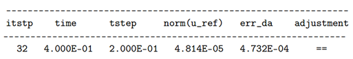
The fields show the current time step number (itstp), current time (time), time stepping size h (tstep), the norm of the reference displacement (u_ref), the acceleration error (err_da) and adjustment request (adjustment), respectively. In particular, the adjustment request field shows two symbols, with the following syntax:
=
|
Indicates no change in h
|
-
|
Indicates a reduction request for h
|
+
|
Indicates an increase request for h
|
==
|
Indicates no change in h for current and subsequent step
|
--
|
Indicates reduction request for h in both current and subsequent step
|
=-
|
Indicates that h remains unchanged for the current step and a reduction request exists for the subsequent step.
|
Note:
| 2. | The NLADAPT entry is recommended to be used to control the maximum and minimum time-step in Nonlinear Transient Analysis. |


