This solution sequence performs quasi-static nonlinear analysis. Quasi-static inherently implies that a process occurring in real-time is being simulated infinitely slowly. This allows the equilibrium equation to be satisfied at each step and inertia, momentum effects are ignored. Therefore the possibly dynamic problem can be solved as a static problem (quasi-static).
Typical Sources of Nonlinearity
Geometric Nonlinearity
In analyses involving geometric nonlinearity, changes in geometry as the structure deforms are considered in formulating the constitutive and equilibrium equations. Many engineering applications require the use of large deformation analysis based on geometric nonlinearity. Applications such as metal forming, tire analysis, and medical device analysis. Small deformation analysis based on geometric nonlinearity is required for some applications, like analysis involving cables, arches and shells. Such applications involve small deformation, except finite displacement or rotation.
Material Nonlinearity
Material nonlinearity involves the nonlinear behavior of a material based on current deformation, deformation history, rate of deformation, temperature, pressure, and so on.
Constraint and Contact Nonlinearity
Constraint nonlinearity in a system can occur if kinematic constraints are present in the model. The kinematic degrees-of-freedom of a model can be constrained by imposing restrictions on its movement. In OptiStruct, constraints are enforced with Lagrange multipliers.
In the case of contact, the constraint condition is based on inequalities and such a constraint generally does not allow penetration between any two bodies in contact.
Follower Load
Applied loads can depend upon the deformation of the structure when large deformations are involved. Geometrically, the applied loads (Forces or Pressure) can deviate from their initial direction based on how the model deforms at the location of application of load. In OptiStruct, if the applied load is treated as follower load, the orientation and/or the integrated magnitude of the load will be updated with changing geometry throughout the analysis.
Types of Nonlinear Quasi-static Analysis
The following analysis types are available in the Quasi-static analysis domain within OptiStruct to solve nonlinear models. Small displacement analysis cannot handle all the nonlinearities specified in the previous section. In such cases, Large displacement analysis can be used. Currently, small displacement analysis is used by default and large displacement analysis can be activated (LGDISP), if required.
Small displacement analysis
In small displacement analysis the sources of nonlinearity are restricted to contact, GAP elements, and MATS1 elastic-plastic material. Geometric nonlinearities, follower loads, and large strain elasto-plasticity cannot be handled by small displacement analysis. As a typical guideline, small displacement analysis should be limited to small strains (some 5 percent strain) in both translation and rotation. There is no update of gap/contact element locations or orientation due to the deformations. They remain the same throughout the nonlinear computations. The orientation may change, however, due to geometry changes in optimization runs. Inertia relief is also supported.
Large displacement analysis
Large displacement nonlinear static analysis (LGDISP) is used for the solution of problems wherein the load response relationship is nonlinear and large structural displacements are involved. The source of this nonlinearity can be attributed to multiple system properties, for example, materials, geometry, nonlinear loading and constraints. Currently, in OptiStruct the large displacement capabilities include large strain elasto-plasticity (MATS1), hyperelasticity of polynomial form (MATHE), contact with small tangential motion, deformation dependent loads (follower loads), and rigid body constraints.
Nonlinear Solution Method
Nonlinear problems are generally history dependent. In order to achieve a certain level of accuracy, the solution must be obtained in a series of small increments. For this purpose you need to solve the equilibrium equation at each increment and a corresponding increment size is selected.
Newton’s method is used to solve the nonlinear equilibrium equation in OptiStruct. If the solution is smooth, quadratic of rate of convergence may be achieved when compared with other methods. This method is also very robust in highly nonlinear situations.
Choosing a suitable time increment is very important. In OptiStruct, an automatic time increment control is available. It should be suitable for a wide range of nonlinear problems and, in general, is a very reliable approach. In future OptiStruct versions, additional user control options to set up automatic time increments may be provided.
The automatic time increment control functionality measures the difficulty of convergence at the current increment. If the calculated number of iterations is equal to optimal number of iterations for convergence, OptiStruct will proceed with the same increment size. If a lesser number of iterations is required to achieve convergence, the increment size will be increased for next increment. Similarly, if it is determined that too many iterations are required, the current increment will be attempted again with a smaller increment size.
The Newton method is used for the solution of nonlinear problems for both Small displacement and Large displacement analysis. The principle of this method is illustrated for a one-dimensional problem in the figure below and can be formulated as follows for small displacement analysis:
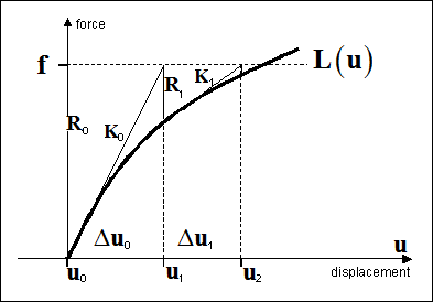
Consider a nonlinear problem:

Where, u is the displacement vector, f is the global load vector, and L(u) is the nonlinear response of the system (nodal reactions). Note that for a linear problem, L(u) would simply be Ku (as described in Linear Static Analysis). Application of Newton's method to this equation leads to an iterative solution procedure:
Where,
In the above formulas, Kn represents a "slope" matrix, defined as a tangent to the L(u) curve at a point un , and Rn is the nonlinear residual. Repeating this procedure iteratively, under certain convergence conditions, leads to systematic reduction of residual Rn and hence, convergence.
| Note: | Specifically only for small displacement nonlinear analysis, that the above scheme is somewhat modified to an equivalent format wherein, instead of calculating  , the new solution un+1 is directly obtained: , the new solution un+1 is directly obtained: |
This form is readily produced by adding Kn un to both sides of Newton's equation, and has certain advantages in practical implementations.
Incremental Loading
For a large class of problems satisfying certain stability and smoothness conditions, the Newton's iterative method is proven to converge, provided that the initial guess is sufficiently close to the true force-displacement path L(u). Hence, to improve convergence for strongly nonlinear problems, the total loading f is often applied in smaller increments, as shown in the figure below. At each of the intermediate loads, f1, f2, and so on, the standard Newton iterations are performed.
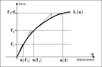
This procedure, known as incremental loading, helps to keep the consecutive iterations closer to the true load path, thereby improving the chances of obtaining a final, converged solution (though usually at the expense of an increased total number of iterations).
Nonlinear Convergence Criteria
In order to assess whether the nonlinear process has converged, a number of convergence criteria are available. These criteria and respective tolerances can be selected on the NLPARM bulk data card. The basic principle in assessing nonlinear convergence is to compare an error measure of the solution with a pre-determined tolerance level. When the error falls below the specified tolerance, the problem is considered converged. In a case of multiple, simultaneous convergence criteria, all criteria need to be satisfied for the solution to be converged.
Relative error in displacements
The relative error in displacements (printed in the convergence summary as EUI) is calculated as:
Where, A is a normalizing vector consisting of square roots of diagonal elements of stiffness matrix K,

and the vector norm is calculated as:
 for small displacement nonlinear analysis and the value of q is calculated as follows:
q is a contraction factor that corrects the increment of solution  to better represent the actual error in the small displacement nonlinear solution. It is expressed as:

In order to stabilize the behavior of q in practical computations, it is updated iteratively according to the formula:
Starting from initial value q1 = 0.99. Note that the contraction factor is meaningful when the solution is close to having converged – it then reasonably estimates the actual error remaining in the small displacement nonlinear solution.
k = 1 for large displacement nonlinear analysis.
Relative error in terms of loads
The relative error in terms of loads (printed in convergence summary as EPI) measures the relative strength of the residual R, and is calculated as:

The load vector f in this formula includes nodal reactions due to specified displacements.
Relative error in terms of work
The relative error in terms of work (printed in convergence summary as EWI) measures the relative change in solution energy, and is calculated as:
Note that the above norms only measure the error of the nonlinear iterative process. Their values do not represent the accuracy of the finite element solution, only the fact that the nonlinear process has converged properly.
Problem Setup
Small Displacement Nonlinear Analysis
The setup for the small displacement nonlinear solution is as shown below. The static loads and boundary conditions are defined in the bulk data section of the input deck. They need to be referenced in the subcase information section using an SPC and LOAD statement in a SUBCASE. Each SUBCASE defines a load vector. Loads or enforced displacements are not mandatory for nonlinear quasi-static solutions, if GAP or CONTACT elements are present in the model.
Unconstrained models can be solved using inertia relief. SUPORT1 subcase statements can then reference the boundary conditions that restrain the rigid body motions. Up to six degrees-of-freedom can be restrained. These restraints can also be defined without subcase reference using the SUPORT bulk data entry or automated using PARAM, INREL, -2.
To indicate that a nonlinear solution is required for any subcase, a subcase information command NLPARM needs to be present for the subcase. This command, in turn, points to the bulk data NLPARM card that contains the convergence tolerances and other nonlinear parameters.
The NLOUT Bulk Data Entry and NLOUT Subcase Information Entry can be used to control incremental output in Small Displacement Nonlinear and Large Displacement Nonlinear Analysis.
Example:
SUBCASE 10
SPC = 1
LOAD = 2
NLPARM = 99
.
.
BEGIN BULK
NLPARM 99 12 UPW+1.1e-5
.
Note that nonlinear gap and contact analysis are also supported in optimization.
Large Displacement Nonlinear Analysis
The setup for the large displacement nonlinear static solution is as follows.
| 1. | PARAM, LGDISP,1 is used to activate large displacement analysis for all subcases containing the NLPARM Subcase Information Entry in the model. Subcase-specific Large Displacement Analysis can be activated via NLPARM(LGDISP)=SID, wherein, SID references a NLPARM Bulk Data Entry. |
| 2. | To indicate that a nonlinear solution is required for any subcase, the NLPARM subcase information entry should be included in the corresponding subcase. |
| 3. | This subcase entry, in turn, references a NLPARM bulk data entry that contains the convergence tolerances and other nonlinear parameters. |
| 4. | NLADAPT bulk/subcase entry can be used to control the number of cutbacks, MAX/MIN time increment. With NLADAPT, you can also add the contact status change in convergence criteria and activate the linear extrapolation in Newton-Raphson method. |
| 5. | If constraints or contacts are defined in the model, the matrix profile may be updated over time, so it is recommended that hash assembly is used for nonlinear analysis. This is activated using PARAM, HASHASSM,YES. |
| 6. | Loads can be treated as Follower loads by using the FLLWER Bulk Data Entry and FLLWER Subcase Information Entry. Additionally, PARAM, FLLWER can be used for global activation/deactivation of Follower Loads. Follower Loads can only be activated for Large Displacement Nonlinear Analysis, consequently, PARAM, LGDISP, 1 (or subcase-specific NLPARM(LGDISP)=SID) should be added to the input file. If a large displacement nonlinear subcase contains a FLLWER subcase entry while PARAM,FLLWER is present in the deck, the follower force calculation parameters defined by the FLLWER bulk data entry (referenced by the FLLWER command) overrides the global follower force settings of PARAM, FLLWER, <-1, 0, 1, 2, 3> for this subcase. |
Follower Forces:
FORCE1/FORCE2 Bulk Data Entries can be used to define follower forces. The OPT field on FLLWER bulk data entry/value on PARAM, FLLWER can be used to control the follower force configuration.
Follower Pressures:
The PLOAD4 Bulk Data Entry can be used to define follower pressure. If the PLOAD4 continuation line is not used, the initial pressure is always directed along the element normal. The OPT field on FLLWER bulk data entry/value on PARAM, FLLWER can be used to control the follower pressure configuration.
Directional Follower Pressure:
The CID, N1, N2, N3 continuation line on PLOAD4 can be used to define directional pressure loading. If directional pressure loading is defined within a follower load case, a local coordinate system, aligned with the material coordinate axis, is constructed. If OPT = 1 or 3 is specified, the pressure holds its initial direction in the local coordinate system. If OPT=2 is specified, the pressure holds its initial direction in the basic coordinate system.
If OPT=1 or 2, for a given PLOAD4 entry, the pressurized area is calculated on the deformed configuration. Otherwise, the pressurized area is calculated on the initial configuration.
Example
PARAM,LGDISP,1
PARAM,FLLWER,1
PARAM,HASHASSM,YES
SUBCASE 10
SPC = 1
LOAD = 2
FLLWER = 31
NLPARM = 99
BEGIN BULK
FLLWER,31
+,LOADSET,-1,101
+,LOADSET,0,102
+,LOADSET,1,103
+,LOADSET,2,104
| 7. | The NLOUT Bulk Data Entry and NLOUT Subcase Information Entry can be used to control incremental output in Small Displacement Nonlinear and Large Displacement Nonlinear Analysis. |
Restart of Nonlinear Analysis
A Nonlinear Analysis run can be restarted or continued from the last point at which the initial run was interrupted (for example, due to a power outage). Illustrated below is the procedure for restarting a nonlinear analysis run with RESTARTW and RESTARTR entries.
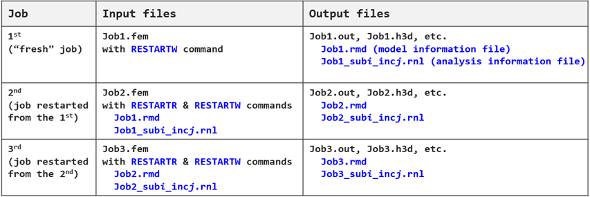
To restart a nonlinear analysis, you will need model information and analysis information of the previous interrupted run. This information is stored in .rmd and .rnl files in binary format.
| • | In an original job with RESTARTW command defined in the input deck, OptiStruct writes one restart model information file (*.rmd) and one or more restart analysis information files (*.rnl) for the nonlinear analysis increments. |
| • | In a restart job with RESTARTR command defined in the input deck, OptiStruct reads a restart model information file (*.rmd) and a restart analysis information file (*.rnl) to retrieve the data needed for restart. |
The input decks of the original and restart runs should be identical except for the RESTARTR and RESTARTW commands.
Note:
| 1. | Large displacement nonlinear analysis is supported for Solid elements, Shell (first order only) elements, CBUSH, RROD, CELASi, RBAR, RBE2, and RBE3 entries. Also, MPC is supported. |
SPC can be applied to the dependent grid on the RBE3 Bulk Data Entry for large displacement analysis.
| 2. | Direct Matrix Input (using the DMIG entry) is currently not supported in large displacement nonlinear analysis, but DMIG is assumed to be small displacement. |
| 3. | Linear Buckling Analysis and Preloaded Analysis are not supported with large displacement nonlinear analysis. |
| 4. | Adaptive load increment technique with the expert system (PARAM, EXPERTNL) is currently not supported with large displacement nonlinear analysis. However, the stabilization with PARAM,EXPERTNL,CNTSTB is supported for large displacement analysis. |
| 5. | Nonlinear Heat Transfer Analysis is currently not supported with large displacement nonlinear analysis. |
| 6. | Large Displacement Nonlinear Analysis is not supported in conjunction with the following elements: |
| (a) | Gasket elements can exist in the model, but they will be resolved using small displacement nonlinear theory (equivalent to ANALYSIS = NLSTAT with plasticity). If large translations or rotations are expected on these elements, the results may not be accurate. |
| (b) | The following elements are not allowed and OptiStruct will error out if they are present: |
CGAP, CGAPG, CWELD, CSEAM, CFAST, RBE1, and CONM
Convergence Considerations for Small Displacement Nonlinear Analysis
For small displacement nonlinear analysis, the Newton's method is a reliable tool for the solution of nonlinear problems and can provide a fast quadratic convergence rate. However, convergence is not guaranteed under all circumstances. Contact problems, especially those with friction, often cause convergence difficulties.
In order to improve the chances of a successfully converged solution, methods have been built in to help problems converge that would otherwise oscillate back-and-forth and never converge. One method involves a "sticky gap," wherein a residual stickiness is introduced to prevent the "undecided" nodes from bouncing in and out of contact. Another method is gap/contact status freezing where, after a number of oscillating iterations, gap/contact elements are not allowed to change their open/closed status. Note that these methods are activated only for near-converging yet stagnated problems, and do not interfere with converging (or radically diverging) cases.
Realistic Problem Setup
Make sure that the nonlinear problem represents a realistic physical situation for which a feasible solution exists. In particular, special care needs to be taken in selecting the proper orientation of gap elements. This is especially important when using a specified gap coordinate system. See the description of the CGAP and CGAPG elements for more details.
Sufficient Support
Since gap/contact elements only provide one-way support, it is possible to formulate the problem in such a way that the individual components will have rigid body freedom under certain loading conditions. This will manifest as zero pivot in the solution process. To avoid such situations, it is advisable to provide sufficient support to all components so that, even without gap/contact elements, there are no rigid body modes. If "solid" supports are not feasible for all parts (the part needs to move), a very weak set of springs can be used to prevent the part from "flying away" when gap/contact elements are not engaged. The stiffness of such auxiliary springs can be selected so as to allow for large motion of the part, compatible with the overall size of the model. If the gap elements and contact interfaces are properly set up, such weak springs will exert virtually no effect when the solution has converged.
Reasonable Gap Stiffness
The gap stiffness values KA and KT essentially represent penalty springs that are hard enough to prevent perceptible penetration of contacting nodes. While, theoretically, higher stiffness values enforce the contact conditions more precisely, excessively high values may cause difficulties in convergence or poor conditioning of the stiffness matrix (this is especially true for KT). If any such symptoms are observed, it may be beneficial to reduce the value of gap stiffness. As a baseline recommendation, a reasonable range of gap stiffness is of the order of:
(103 to 106) * E * h
Where, E is the typical value of elastic modulus and h is the typical element size in the area surrounding the gap elements. Such range will generally keep the gap penetration below one thousandth/one millionth of the element size, respectively. A good value for KT is of the order of 0.1*KA.
To facilitate reasonable values of KA and KT, OptiStruct supports the automatic calculation of these parameters, specifically:
| • | Option KA=AUTO determines the value of KA for each gap element using the stiffness of surrounding elements. Additional options SOFT and HARD create respectively softer or harder penalties. SOFT can be used in cases of convergence difficulties and HARD can be used if undesirable penetration is detected in the solution. |
| • | Option KT=AUTO automatically calculates the value of KT. If MU1>0, the result here is the same as with blank KT -- its value is calculated as MU1*KA. However, if MU1=0 or blank, KT=AUTO produces a non-zero value of KT, calculated as KT=0.1*KA. Therefore, KT=AUTO can be used to specify enforced stick conditions. |
Friction
The presence of friction, due to its strong nonlinear, non-conservative nature, may cause difficulties in nonlinear convergence, especially when sliding is present. Therefore, solving the problem without friction can often provide convergence in otherwise failing problems. Or, in cases when presence of frictional resistance is necessary and minimal sliding is expected, enforcing a stick condition may be a viable solution, and will often lead to a better convergence than Coulomb friction (refer to the PGAP and PCONT bulk data cards for details). In cases of larger sliding motions, the stick condition may lead to divergence through a "tumbling" mode.
Gap Offset
In order to provide theoretical correctness, friction produces bending moments in gap/contact elements of non-zero length (this results from the transfer of frictional force from the contact surface to the end nodes). This offset operation can, however, cause convergence problems and counter-intuitive results. In problems with friction, it may be advisable to turn off the offset operation via a parameter:
GAPPRM,GAPOFFS,NO
This will produce more intuitive results in the presence of friction. However, it may violate the rigid body balance of the body, and should therefore be used with caution, especially for problems without full SPC support. Refer to the PGAP and PCONT bulk data cards for details.
Incremental Loading
If the nonlinear procedure diverges, in spite of taking the measures described above, the incremental loading procedure (applying the total load in a number of increments) can be used to achieve convergence. Refer to the NLPARM bulk data card for details. Note, however, that if the problem is incorrectly formulated (the solution exhibits excessive deformations, free rigid body motions, an ill-conditioned stiffness matrix, extremely high nonlinear error, etc.), incremental loading cannot be counted on to provide a converged solution.
Nonlinear Expert System
In some difficult to converge cases, an expert system can be used to achieve convergence:
PARAM,EXPERTNL,YES
The expert system will try to adjust the load increment and other nonlinear parameters to achieve convergence. Note, however, that if the problem is incorrectly formulated (the solution exhibits excessive deformations, free rigid body motions, an ill-conditioned stiffness matrix, extremely high nonlinear error, etc.), expert system cannot be counted on to provide a converged solution.
Moreover, in some cases it can lead to long computational times without success. This may be due to using very small load increments or re-running the solution with modified nonlinear parameters.


