Geometric nonlinear analysis in OptiStruct is provided through an integration of the RADIOSS Starter and RADIOSS Engine via a translator. Implicit (static and dynamic), as well as explicit integration schemes, are available. Transparent to you, OptiStruct input data is directly translated into RADIOSS input data. The RADIOSS Starter and RADIOSS Engine are then executed and the results are brought back into the OptiStruct output module to export the different output formats.
Solution Method
This section covers the basic concepts of the solution methods to highlight the characteristics of the solution methods and to identify the use of certain parameters to control convergence. The geometric nonlinear solution utilizes a general Newmark integration scheme. The following equation of motion shall be solved.
The matrix M is the mass matrix, C is the damping matrix and K is the stiffness matrix. These matrices are derived using finite elements. The vector P describes the external loads and u is the displacement vector. The dots describe the derivatives with respect to time.
The equation of motion can be solved using a general Newmark integration scheme. Newmark is a one-step time integration method. All solutions can be derived from it and are formulated in terms of a time history (Figure 1).
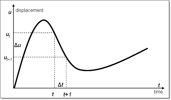
Figure 1: Time History
In general Newmark, the state vector is computed as follows:
Then the equation of motion yields:

This can be rewritten into:
using:
In short:

The matrix A is the dynamic stiffness. In nonlinear time-dependent problems, this system becomes nonlinear and its solution requires an additional iteration loop at each time step using a Newton-type method.
An implicit (quasi-)static analysis scheme follows directly when omitting mass and damping terms. Therefore:
The linear static case reduces to the systems equation:
Ku = P
Normal modes analysis is a linear analysis that solves the eigenvalues problem.
For implicit dynamic analysis, an extension of Newmark method, known as a-HHT, is the default time integrator. This method is named after Hilber, Hughes, and Taylor – it allows for effective algorithmic damping of high-frequency spurious vibrations. This method introduces additional parameter a and assumes:
The smaller the value of a, the more algorithmic damping is included in the numerical solution. With a = 0.0, there is no numerical damping and the method is the trapezoidal method.
The second method available is the general Newmark with user-defined  and
and  . The defaults are typically:
which is equivalent to HHT method with a = 0.0. This is an unconditionally stable implicit integration scheme with:
And from the equation of motion:
By default a Modified Newton method is employed to solve the implicit problems stated above (Figure 2).
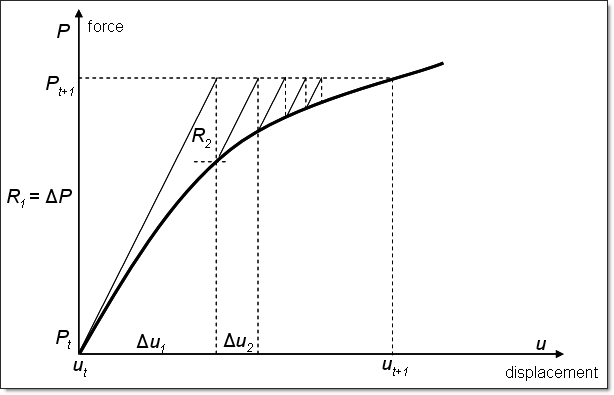
Figure 2: Implicit scheme
Convergence for implicit (quasi-)static and dynamic analysis is controlled via NLPARM and TSTEPNL bulk data entries, respectively. Modified Newton requires that the stiffness matrix is kept constant through a number of iterations (KSTEP) before it is rebuilt. This saves computation time in terms of matrix factorizations, but may increase the number of iterations. Full Newton can be achieved by using KSTEP = 1.
Convergence is defined by a change in results less than a specified tolerance. Relative residual force (EPSP), relative displacement (EPSU), or relative residual energy (EPSW) can be chosen as convergence criteria (CONV).
In implicit analysis the time step is controlled via NLPARMX and TSTEPNX bulk data entries, respectively. Time step control includes a minimum (DTMIN) which terminates the solution, a maximum (DTMAX) time step, as well as a maximum number of time steps which cannot be exceeded. Using convergence acceleration methods (SACC), more control can be asserted. If the number of iterations within a time step reaches a specified limit (LDTN), the iteration is repeated with a smaller time step. The time step is also reduced should the iteration diverge. If the number of iterations is below a certain limit (ITW), the time step is increased.
A BFGS Quasi-Newton method is also available to solve the implicit equations. It works similarly to Modified Newton. However, in addition to the tangential stiffness, it uses an approximate Hessian to improve convergence.
A conditionally stable explicit integration scheme can be derived from the Newmark scheme by setting:
From these relationships the central differences explicit integration scheme can be derived.
Figure 3 illustrates the relationships.
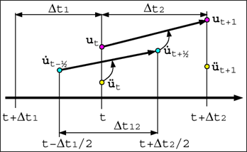
Figure 3: Explicit integration
Assuming that
The equation of motion for the central differences scheme simplifies to:
This central differences scheme is used if explicit analysis is selected. The time step must always be smaller than the critical time step to ensure stability of the solution. The critical time step depends on the highest frequency in the system and is computed from the corresponding angular frequency  max as:
For a discrete system, the time step must be small enough to excite all frequencies in the finite element mesh. This requires such a short time step that a shock wave does not miss any node when traveling the mesh. Therefore,

with lc being the critical length of an element and c is the speed of sound in the given material.
Different ways of time step control are available. The default method is the nodal time step which is computed from the nodal mass m and the equivalent nodal stiffness k such that:
The element time step based on the critical length of each element is also available. The choice can be made on the XSTEP bulk data entry.
Problem Setup
Geometric nonlinear analysis is defined through a SUBCASE.
For implicit (quasi-)static analysis an NLPARM statement as well as ANALYSIS = NLGEOM must be present in the subcase. To define the termination time, a TTERM subcase entry can be used. TTERM is mandatory if a nonlinear load NLOAD is used. NLPARM references an NLPARM bulk data entry. Additional parameters to control the geometric nonlinear solution can be defined on the optional NLPARMX bulk data entry. These include convergence acceleration methods. In the case of post-buckling analysis, Riks method can be selected.
Linear static analysis is provided as a debugging option. It is defined through NLPARMX, ILIN. Such analysis can help investigate the model for modeling errors. In linear static analysis, the load vector is determined at the termination time. Normal modes analysis requires a METHOD subcase statement in addition.
For implicit dynamic analysis a TSTEPNL statement as well as ANALYSIS = IMPDYN must be present in the subcase. To define the termination time a TTERM subcase entry is mandatory. TSTEPNL references a TSTEPNL bulk data entry. Additional parameters to control the geometric nonlinear solution can be defined on the optional TSTEPNX bulk data entry.
For explicit dynamic analysis an XSTEP statement as well as ANALYSIS = EXPDYN must be present in the subcase. To define the termination time a TTERM subcase entry is mandatory. XSTEP references an XSTEP bulk data entry. Time step control can be defined on the XSTEP bulk data entry.
The implicit schemes require the solution of linear systems equations. By default, the direct solver is invoked, whereby the unknowns are simultaneously solved using a Gauss elimination method that exploits the sparseness and symmetry of the stiffness matrix, K, for computational efficiency. Alternatively, an iterative solver using the preconditioning conjugate gradient method may be used. While the direct solver is very robust, accurate and efficient, the iterative solver is sometimes superior in terms of speed, for example for bulky solid structures. The iterative solver is selected through the SOLVTYP subcase information entry, which in turn references a SOLVTYP bulk data entry.
The definition of a unit system through the DTI, UNITS or UNITS bulk data statement is required.
The geometric nonlinear analysis loads and boundary conditions are defined in the bulk data section of the input deck. They need to be referenced under the SUBCASE using an SPC, NLOAD, LOAD, IC and RWALL statements in a SUBCASE. Each SUBCASE defines one loading condition that is executed separately.
Subcase continuation is available through the use of CNTNLSUB. Any number of explicit and implicit analyses can be linked. However, geometric nonlinear (ANALYSIS = NLGEOM, EXPDYN, or IMPDYN) analysis subcases cannot yet be linked with small displacement quasi-static nonlinear (ANALYSIS = NLSTAT) analysis subcases and vice versa.
SUBCASE 1
ANALYSIS = NLGEOM
SPC = 1
NLOAD = 2
NLPARM = 3
TTERM = 1.0
DISP = ALL
STRESS = ALL
BEGIN BULK
NLPARM,3
NLOAD1,2,2,,L,88
TABLED1,88,
+,0.0,0.0,1.0,1.0,ENDT
DTI,UNITS,1,kg,N,m,s
|
SUBCASE 1
ANALYSIS = NLGEOM
SPC = 1
LOAD = 4
NLPARM = 3
DISP = ALL
STRESS = ALL
BEGIN BULK
NLPARM,3
FORCE,4,233,,1.0,0.0,0.0,1.0
DTI,UNITS,1,kg,N,m,s
|
SUBCASE 2
ANALYSIS = IMPDYN
SPC = 1
IC = 5
TSTEPNL = 3
TTERM = 0.2
DISP = ALL
STRESS = ALL
BEGIN BULK
TSTEPNL,3
TIC,5,123,1,,13.88
DTI,UNITS,1,kg,N,m,s
|
SUBCASE 3
ANALYSIS = EXPDYN
SPC = 1
NLOAD = 2
XSTEP = 3
TTERM = 1.0
DISP = ALL
STRESS = ALL
BEGIN BULK
XSTEP,3
NLOAD1,2,2,,L,88
TABLED1,88,
+,0.0,0.0,1.0,1.0,ENDT
DTI,UNITS,1,kg,N,m,s
|
DISP = ALL
STRESS = ALL
SUBCASE 1
ANALYSIS = NLGEOM
SPC = 1
NLOAD = 2
NLPARM = 3
TTERM = 1.0
SUBCASE 2
ANALYSIS = EXPDYN
IC = 5
XSTEP = 4
TTERM = 1.1
CNTNLSUB = 1
BEGIN BULK
NLPARM,3
XSTEP,4
NLOAD1,2,2,,L,88
GRAV,2,,9.81,0.0,0.0,1.0
TABLED1,88,
+,0.0,0.0,1.0,1.0ENDT
TIC,5,123,1,,13.88
DTI,UNITS,1,kg,N,m,s
|
DISP = ALL
STRESS = ALL
ANALYSIS = NLGEOM
CNTNLSUB, YES
SUBCASE 1
SPC = 1
LOAD = 2
NLPARM = 3
SUBCASE 2
SPC = 1
LOAD = 4
NLPARM = 3
BEGIN BULK
NLPARM,3
GRAV,2,,9.81,0.0,0.0,1.0
FORCE,4,233,,1.0,0.0,0.0,1.0
UNITS = SI
|
User's Considerations
Geometric Nonlinear Analysis Properties and Materials
Special element types and nonlinear materials are available for geometric nonlinear analysis. As a general rule property and material definitions that are only applicable in geometric nonlinear analysis are defined on extensions to the original property and to a MAT1 material, respectively. The extensions are grouped with the base entry by sharing the same PID or MID. In the case of a subcase that is not a geometric nonlinear analysis, these extensions are ignored. Property defaults can be set for shells (XSHLPRM) and solids (XSOLPRM) that may replace the use of property extensions.
Property example:
PSHELL, 3, 7, 1.0, 7, , 7
PSHELLX, 3, 24, , , 5
Material example:
MAT1, 102, 60.4, , 0.33, 2.70e-6
MATX02, 102, 0.09026, 0.22313, 0.3746, 100.0, 0.175
Coordinate Systems
In geometric nonlinear analysis there are moving and fixed coordinate systems. Rectangular coordinate systems that are defined through grid points (CORD1R, CORD3R) are moving with the deformations of the model. Systems defined in terms of point coordinates (CORD2R, CORD4R) are fixed.
The behavior of loads depends on the coordinate system referenced. If the loads FORCE and MOMENT are desired to be follower forces, a CID that references a moving coordinate system (CORD1R, CORD3R) must be defined. Otherwise these loads are not following the deformation. PLOAD always follows the deformations.
Difference Between Geometric Linear and Geometric Nonlinear Analysis
In geometric linear analysis all deformations and rotations are small (infinitesimal). As a general rule, displacements of say 5% of the model dimension and rotations up to 5 degrees can be treated as small. Rotations are trickier. A rotating body seems to get bigger linearly under deformation even if defined as rigid. Nonlinearities can only come from contact or materials. This type of analysis is supported in Small Displacement Nonlinear Analysis with ANALYSIS = NLSTAT. Loads stay in the undeformed coordinates and simply move along the axis they are defined in.
In geometric nonlinear analysis, displacements and rotations are large (finite). The magnitude of a force actually matters. Changes in magnitude of a load can change convergence behavior considerably. Also the direction of a force needs to be controlled. Forces may follow the deformation or keep their direction. This can be controlled through the choice of coordinate systems (see above).
The images below display two examples of these differences. Figure 4 shows a cantilever beam solved with small displacements, large displacements with a follower force, and large displacements without a follower force. Figure 5 shows a simple rigid rotated by an angle  solved with small and finite rotations.
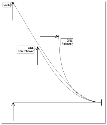
Figure 4: Cantilever beam with small (GLIN) and large (GNL) displacements
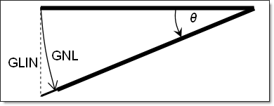
Figure 5: Small (GLIN) vs. finite (GNL) rotations
Difference Between Implicit and Explicit Analysis
Implicit static analysis has the following characteristics:
| • | Involves matrix factorization |
| • | Stiffness matrix must be positive definite |
| - | Model must be sufficiently constraint |
| • | Iteration is needed to reach equilibrium |
| • | Equilibrium is achieved within iteration tolerances |
| • | Long-term, (quasi-)static events |
Implicit dynamic analysis has the following characteristics:
| • | Involves matrix factorization |
| • | Dynamic stiffness matrix must be positive definite |
| • | Iteration is needed to reach equilibrium |
| • | Equilibrium is achieved within iteration tolerances |
Explicit (dynamic) analysis has the following characteristics:
| • | In general a diagonal mass matrix is used |
| • | No matrix factorization necessary |
| • | Equilibrium is always guaranteed |
| • | Maximum stable time step needs to be respected |
Implicit Contact
In an implicit contact analysis, you need to take care of the following two concerns:
First, there should be no initial penetrations in the mesh. Sometimes, initial penetration is necessary to begin the simulation then only a small (< 0.01*GAP) value is recommended to not change reality too much. With high initial penetrations, the solution will progress but may lead to incorrect results. You will be warned about initial penetration during the check run.
Secondly, in quasi-static analysis the model needs to be sufficiently constrained. For example, having two blocks on top of each other (Figure 6) the top part is not constrained. It is recommended to have the meshes completely depenetrated and to define a very small GAP. This would create small springs constraining the upper body in vertical direction. Of course, the other rigid body motions of the part have to be constrained too.
More information can be found in CONTACT, CONTPRM, and PCONTX bulk data definitions.
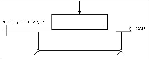
Figure 6: Initial GAP
Implicit Snap-thru, Post-buckling Analysis
Some nonlinear problems with large deformations encounter bifurcations. The solution becomes instable and the structure buckles or snaps from one state to another (Figure 7). The load vs. displacement does not simply increase but may reduce until another stable point is reached from which the load can then continue to increase (Figure 8). In the implicit solution procedure it is clear that a simple load increment may not be sufficient to determine the point where the force starts reducing.
A special method needs to be employed to find the proper search direction  s for the solution to stay on its path. This solution is called Riks method and can be defined via NLPARMX, SACC. The search direction is defined by satisfying certain constraints of which two methods can be selected via NLPARMX, CTYP.
There are currently some limitations in the way the results are written. Internal forces cannot be plotted yet.
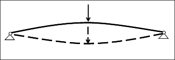
Figure 7: Snap-thru
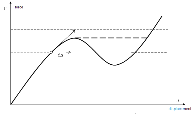
Figure 8: Snap-thru - Load vs. displacement
Insufficiently Constrained Model in Implicit (Quasi-)static Analysis
For models that are not sufficiently constrained, inertia stiffness can be used to overcome a singular stiffness matrix (NLPARMX, KINER = ON). The inertia stiffness, Kinertia = 1 / (DTSCQ * dt)2M, is added to the stiffness matrix K in a (quasi-)static analysis. Care needs to be taken in the selection of DTSCQ. An added mass that is too large may lead to incorrect results. This function is similar to inertia relief in other analysis types.
Implicit Convergence Issues
If the iteration process stops with TIME STEP LIMIT ERROR, this indicates the time step has reached DTMIN. In this case, the following measures can be taken to remedy the situation:
Implicit (Quasi-)static
| • | Check if there is any rigid motion by launching a linear run or eigenvalue analysis. |
| • | Double-check the values and units of input parameters (material properties, loads, etc). It is usually helpful to view the results of intermediate animation outputs. |
| • | Increase the number of load increments (NLPARM, NINC), decrease minimum time step (NLPARMX, DTMIN), and/or decrease maximum time step (NLPARMX, DTMAX). |
| • | If post-buckling happens, activate RIKS method (NLPARMX, TSCTRL = RIKS). |
| • | Check the displacement, force and energy residual values during the iteration in the .out file, find out which convergence criteria is causing the divergence, and then modify convergence control criteria (NLPARM, CONV) and relax the tolerances (NLPARM, EPSU, EPSW, and EPSP). It must be understood that reducing the convergence tolerance may lead to inaccurate results. |
| • | Use small displacement formulation (PARAM, SMDISP, 1) if the displacements and rotations are small. |
Implicit Dynamic
| • | Double-check the values and units of input parameters (material properties, loads, etc.). It is usually helpful to view the results of intermediate animation outputs. |
| • | Decrease the initial time step (TSTEPNL, NX), decrease minimum time step (TSTEPNX, DTMIN), and/or decrease maximum time step (TSTEPNX, DTMAX). |
| • | Check the displacement, force and energy residual values during the iteration in the .out file, find out which convergence criteria is causing the divergence, and then modify convergence control criteria (NLPARM, CONV) and relax the tolerances (NLPARM, EPSU, EPSW, and EPSP). It must be understood that reducing the convergence tolerance may lead to inaccurate results. |
| • | Use small displacement formulation (PARAM, SMDISP, 1) if the displacements and rotations are small. |
Limitations
The solution will be terminated if unsupported Bulk Data entries are encountered.
| • | The following Bulk Data properties and elements are currently not translated: |
| - | PBUSHT (partially, KN is translated) |
| - | PGAP, CGAP, CGAPG (partially, friction is not allowed) |
| • | Additional relevant Bulk Data entries (except loads) that are currently not translated: |
| - | MAT2, MAT4, MAT5, MAT8, MAT9, MAT10 |
| • | Relevant loads that are currently not translated: |
| - | PLOAD4 (partially, N1, N2, N3 cannot be used) |
| - | RFORCE (partially, RACC is not supported) |


