OS-4000: 3D Size Optimization of a Rail Joint

This tutorial demonstrates how to perform a size optimization on an automobile rail joint modeled with shell elements. The structural model with loads and constraints applied is shown in the figure below. The deflection at the end of the tubular cross-member should be limited. The optimal solution would be to use as little material as possible.

4000_structural_model

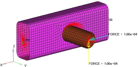
Structural model of a rail joint.

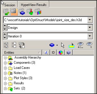
The structural model, shown above, is loaded into HyperMesh. The constraints, loads, material properties, and subcases (loadsteps) are already defined in the model. Size design variables and optimization parameters are defined, and OptiStruct determines the optimal gauges for the components. The results are then reviewed in HyperView.

The optimization problem for this tutorial is stated as:

Objective:	Minimize volume.
Constraints:	A given maximum nodal displacement at the loading grid point for two loading conditions.
Design variables:	Gauges of the two parts.

In this tutorial, you will learn to:

•	Setup a size optimization in HyperMesh

•	Post-process size optimization results in HyperView

Exercise

Set up a Size Optimization in HyperMesh Desktop

Step 1: Launch the HyperMesh Desktop, set the User Profile and Retrieve the File

1.	Launch HyperMesh Desktop.

2.	Choose the OptiStruct in the User Profiles dialog and click OK. This loads the user profile. It includes the appropriate template, macro menu, and import reader, paring down the functionality of HyperMesh to what is relevant for generating models for OptiStruct.

User Profiles GUI can also be accessed from the Preferences menu on the toolbar.

3.	Select the Open Model file toolbar icon .

4.	Select the joint_size.hm file you saved to your working directory from the optistruct.zip file. Refer to Accessing the Model Files.

5.	Click Open.

Step 2: Create the Size Design Variables for Optimization

1.	From the Analysis page, select the optimization panel.

2.	Click the size panel.

3.	Make sure the desvar subpanel is selected using the radio buttons on the left-hand side of the panel.

4.	Click desvar = and enter tube.

5.	Click initial value = and enter 1.0.

6.	Click lower bound = and enter 0.1.

7.	Click upper bound = and enter 5.0.

8.	Make sure the move limit toggle is set to move limit default.

9.	Make sure the discrete design variable (ddval) toggle is set to no ddval.

10.	Click create.

A design variable, tube, has been created. The design variable has an initial value of 1.0, a lower bound of 0.1, and an upper bound of 5.0.

11.	Repeat steps 4 through 10 to create the design variable rail using the same initial value, lower, and upper bounds.

A design variable, rail, has been created. The design variable has an initial value of 1.0, a lower bound of 0.1, and an upper bound of 5.0.

12.	Select the generic relationship subpanel using the radio buttons on the left-hand side of the panel.

13.	Click Name = and enter tube_th.

14.	Click prop and select tube2 from the list of property collectors.

15.	Make sure the toggle is set to Thickness T.

16.	Click designvars. The list of design variables appears.

17.	Check the box next to tube.

Note the linear factor (value is box beside tube) automatically gets set to 1.000.

18.	Click return.

19.	Click create.

A design variable to property relationship, tube_th, has been created relating the design variable tube to the thickness entry on the PSHELL card for the property tube2.

20.	Repeat steps 13 through 19 to create the design variable to property relationship rail_th relating the design variable rail to the thickness entry on the PSHELL card for the property tube1.

21.	Click return to go to the optimization panel.

Step 3: Create the Volume and Static Displacement Response

A detailed description can be found in the OptiStruct User's Guide under Responses.

1.	Enter the responses panel.

2.	Click response = and enter volume.

3.	Click the response type: switch and select volume from the pop-up menu.

4.	Ensure the regional selection is set to total (this is the default).

5.	Click create. A response, volume, is defined for the total volume of the model.

6.	Click response = and enter X_Disp.

7.	Click the response type: switch and select static displacement from the pop-up menu.

8.	Click nodes and select by id from the pop-up menu.

9.	Enter 3143 (node at center of rigid spider at loading point) and press ENTER.

10.	Select dof1 and click create. A response, X_Disp, is defined for the x-displacement of the node 3143.

11.	Click response = and enter Z_Disp.

12.	Click nodes and select by id from the pop-up menu.

13.	Enter 3143 (node at center of rigid spider at loading point) and press ENTER.

14.	Select dof3 and Click create. A response, Z_Disp, is defined for the z-displacement of the node 3143.

15.	Click return to go to the optimization panel.

Step 4: Create Constraints on Displacement Response

A response defined as the objective cannot be constrained. In this case, you cannot constrain the response volume.

Upper bound constraints are to be defined for the responses X_Disp and Z_Disp.

1.	Enter the dconstraints panel.

2.	Click constraint = and enter Disp_X.

3.	Check the box for upper bound =.

4.	Click upper bound = and enter 0.9.

5.	Click response = and select X_Disp from the list of responses. A loadsteps button appears in the panel.

6.	Click loadsteps.

7.	Check the box next to FORCE_X and click select.

8.	Click create.

A constraint is defined on the response X_Disp. The constraint is an upper bound with a value of 0.9. The constraint applies to the subcase FORCE_X.

9.	Click constraint = and enter Disp_Z.

10.	Check the box for upper bound =.

11.	Click upper bound = and enter 1.6.

12.	Click response = and select Z_Disp from the list of responses.

13.	Click loadsteps.

14.	Check the box next to FORCE_Z and click select.

15.	Click create.

A constraint is defined on the response Z_Disp. The constraint is an upper bound with a value of 1.6. The constraint applies to the subcase FORCE_Z.

16.	Click return to go to the optimization panel.

Step 5: Define the Objective Function

In this example, the objective is to minimize the volume response defined in the previous section.

1.	Click objective to enter the panel.

2.	The switch in the left should be set to min.

3.	Click response = and select volume from the response list.

4.	Click create. The objective function is now defined.

5.	Click return to go to the optimization panel.

Step 6: Save the HyperMesh Database

1.	From the File menu, select Save as > Model. A Save As dialog appears.

2.	Select the directory where you would like to save the database and enter the name for the database, joint_sizeOPT.hm, in the File name: field.

3.	Click save.

Step 7: Run the Optimization Problem

1.	From the Analysis page, select the OptiStruct panel.

2.	Click save as.

3.	Select the directory where you would like to write the model file and enter the name for the file name, joint_sizeOPT.fem, in the File name: field. The .fem file extension is used for OptiStruct input decks.

4.	Click Save.

The name and location of the joint_sizeOPT.fem file displays in the input file: field.

5.	Set the export options: toggle to all.

6.	Click the run options: switch and select optimization.

7.	Set the memory options: toggle to memory default.

8.	Click OptiStruct to run the optimization. This launches the OptiStruct job.

If the job was successful, new results files can be seen in the directory where the OptiStruct model file was written. The joint_sizeOPT.out file is a good place to look for error messages that will help to debug the input deck if any errors are present.

Important files for size optimization include:

joint_sizeOPT.hgdata	HyperGraph file containing data for the objective function, percent constraint violations and constraint for each iteration.
joint_sizeOPT.prop	OptiStruct property output file containing all updated property data from the last iteration for size optimization.
joint_sizeOPT.hist	OptiStruct iteration history file, containing the iteration history of the objective function and of the most violated constraint. This file can be used for a xy plot of the iteration history.
joint_sizeOPT.out	OptiStruct output file containing specific information on the file setup, the setup of the optimization problem, estimates for the amount of RAM and disk space required for the run, information for all optimization iterations, and compute time information. This file contains compliance, volume calculations, and gauge information for all optimization iterations. It is highly recommended to review this file for warnings and errors.
joint_sizeOPT.res	HyperMesh binary result file.
joint_sizeOPT_des.h3d	HyperView binary result file, containing the design iteration results.
joint_sizeOPT_s1.h3d	HyperView binary result file, containing the analysis results of subcase with ID 1.
joint_sizeOPT_s2.h3d	HyperView binary result file, containing the analysis results of subcase with ID 2.
joint_sizeOPT.stat	Summary of analysis process, providing CPU information for each step during analysis process.

Post-process Size Optimization Results in HyperView

Displacement and stress results are output by OptiStruct (by default) for linear static analyses. This section describes how to view those results in HyperView. Size optimization results from OptiStruct are given in the .h3d files and joint_sizeOPT.out.

joint_sizeOPT_des.h3d	Contains the element thickness for all five iterations.
joint_sizeOPT_s1.h3d	Contains displacement and stress results for the linear static analysis for iteration 0 and iteration 4 of subcase with ID 1 (subcase Force_X).
joint_sizeOPT_s2.h3d	Contains displacement and stress results for the linear static analysis for iteration 0 and iteration 4 of subcase with ID 2 (subcase Force_Z).
joint_sizeOPT.out	Contains gauge and volume information for all iterations.

The results contained in the HyperView binary results file will be examined first. Then the gauge history in the joint_sizeOPT.out file will be reviewed.

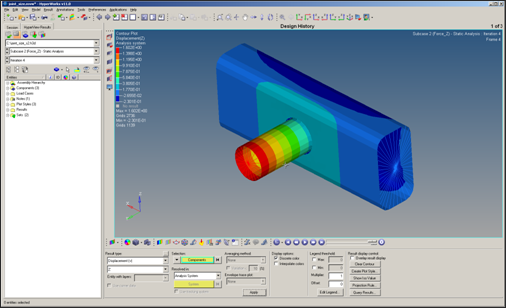
Step 8: View the Size Optimization Results (gauge thickness)

1.	When the message Process completed successfully appears in the command window, click HyperView.

HyperView launches and the results are loaded. A message window appears to inform about the successful loading of the model and result files into HyperView. Notice that all three .h3d files get loaded, each into a different page in HyperView. The files joint_sizeOPT_des.h3d, joint_sizeOPT_s1.h3d, and joint_sizeOPT_s2.h3d get loaded in page 2, page 3, and page 4, respectively. The optimization iteration results (gauge thickness) are loaded in the first page. The name of the page is displayed as Design History to indicate that the results correspond to optimization iterations.

2.	Click Close to close the message window.

3.	Click the Contour toolbar icon .

4.	Make sure the first drop-down list below Result type: is on Element Thicknesses (s).

5.	Make sure the second drop-down list is set to Thickness.

6.	Make sure the field below Averaging method is None.

7.	Set the last load case simulation in the HyperView Results browser, as shown below. Scroll down to choose the last iteration (Iteration 4, in this case), and click OK.

os_4000_hvresults_tab

8.	Click Apply.

A contoured image representing shell thickness should be visible. Each element in the model is assigned a legend color, indicating the thickness value for that element for the current iteration.

4000_thickness_contour

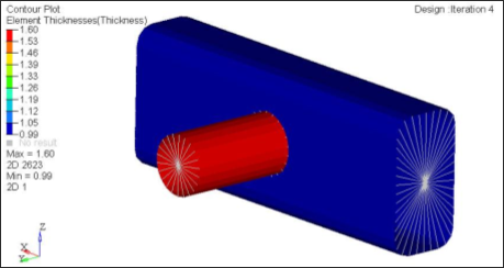
Thickness contour at last iteration.

Step 9: View the Displacement Results

It is helpful to view the deformations of the model to determine if the boundary conditions have been met and also to see if the model is deforming as expected. These analysis results are available in pages 3 and 4.

1.	Click the Next Page toolbar icon .

The third page, which has results loaded from the file joint_sizeOPT_s1.h3d, is displayed. The name of the page is displayed as Subcase 1 – FORCE_X to indicate that the results correspond to subcase 1.

2.	Set the animation mode to Linear Static.

3.	Click the Contour toolbar icon .

4.	Select the first drop-down list below Result type: and select Displacement [v].

5.	Select the second drop-down list and select X.

6.	Click Apply. The resulting contours represent the x component displacement field resulting from the applied loads and boundary conditions.

7.	Click the Measure toolbar icon .

8.	Click Add to add a new measure group. The Measure panel helps measure different results. Here, you will measure the displacement at node 3143 for which you have constrained the displacement.

9.	Click the drop-down menu and select Nodal Contour as shown below.

10.	Click Nodes, which opens a new window to select nodes By ID.

11.	Click By ID to open a new window.

12.	Enter 3143 in the field next to Node ID and click Ok.

os_4000_first_iteration

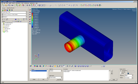
Displacement on X-direction for the X-force loadcase at the first iteration.

The x-displacement value for 3143 (center of rigid spider, where loading is applied) is shown in the graphic area. The x-displacement is larger than the upper bound constraint, which was defined earlier, of 0.9.

13.	In the HyperView Results browser, select the last iteration by double-clicking on the last Iteration #.

The contour now shows the x-displacement results for Subcase 1 (FORCE_X) and iteration 4, which corresponds to the end of the optimization iterations. Note that the x-displacement is now less than 0.9.

os_4000_last_iteration

Displacement on X-direction for the X-force loadcase at the last iteration.

14.	Click the Next Page icon again to move to the fourth page.

The fourth page shows results loaded from the joint_sizeOPT_s2.h3d file. The name of the page is displayed as Subcase 2 – Force_Z to indicate that the results correspond to subcase 2.

15.	Click the Contour toolbar icon .

16.	Select the first drop-down menu below Result type: and select Displacement [v].

17.	Select the second drop-down menu and select Z.

18.	Click Apply. The resulting contours represent the z component displacement field resulting from the applied loads and boundary conditions.

19.	Repeat steps 8 through 14 to measure and display the z-displacement value for node 3143.

os_4000_z_disp

Alternate Way to View the Gauge Thickness Results

From the UNIX or MSDOS shell, open the joint_sizeOPT.out file in a text editor. Review all five iterations, noting the volume, constraint information, and gauge at each iteration.

Has the volume been minimized for the given constraints?

Have the displacement constraints been met?

What are the resulting gauges for the rail and tube?