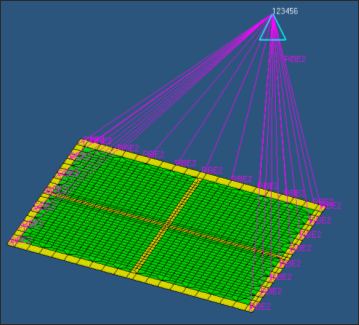
OS-3030: Random Response Optimization

A topography optimization with random response is performed on a flat plate in this tutorial. A random response analysis has been set up. As shown in the following image, the flat panel is constrained through an RBE2 element. Two frequency-varying accelerations are applied on the independent node of the RBE2 element as excitations. They are correlated through a cross-spectral density. The objective of the optimization is to minimize the maximum (minmax) Power Spectral Density (PSD) acceleration in X direction at the center of the panel.

3030_model

Model review

The following exercises are included:

•	Create a topography optimization with PSD response in HyperMesh

•	Submit the job to OptiStruct

•	Post-process the results in HyperView and HyperGraph

Exercise

Load the Model in HyperMesh

Step 1: Load the OptiStruct User Profile and Import the Model

1.	Launch HypferMesh.

2.	Choose OptiStruct in the User Profiles dialog and click OK. This loads the OptiStruct user profile. It includes the appropriate template, macro menu, and import reader, paring down the functionality of HyperMesh to what is relevant for generating OptiStruct models.

User Profiles can also be accessed from the Preferences menu on the toolbar.

3.	Click the Import panel toolbar icon . The File type: is OptiStruct.

4.	Click the open file icon . A Select OptiStruct file browser window opens.

5.	Select the panel.fem file you saved to your working directory from the optistruct.zip file. Refer to Accessing the Model Files.

6.	Click Open. The location of panel.fem displays in the file: field.

7.	Click Import. The panel.fem database is loaded into the current HyperMesh session.

Create Random Response Optimization

Step 2: Create design variables for topography optimization

In this exercise, the design space is composed of the shell elements with the property PSHELL_5. A minimum bead width of 0.4, a bead height of 1, and draw angle of 60 degrees is used in the bead definition. A 2-plane symmetrical pattern grouping constraint is defined to generate a symmetrical bead design.

1.	From the Analysis page, enter the optimization panel.

2.	Click topography to enter the Topography Optimization panel.

3.	Select the create subpanel by clicking the radio button on the left side of the panel.

4.	Click desvar = and enter plate.

5.	Click the highlighted props.

6.	Check the box next to PSHELL_5 and click select.

7.	Click create to create the topography design variable.

8.	Select the bead params subpanel using the radio button.

9.	Click desvar= and select plate.

10.	Enter the bead parameters, as shown in the following image.

3030_bead_params

11.	Click update.

12.	Select the pattern grouping subpanel using the radio button.

13.	Click desvar= and select plate.

14.	Under pattern type:, click on the switch and select 2-plns sym.

15.	For anchor node, first node and second node, click the switch to change from node id to coordinates.

16.	Enter the values as shown below to define a 2-plane symmetry constraint.

3030_2_pln_sym

17.	Click update.

18.	Go to the bounds subpanel using the radio button.

19.	Set Upper Bound = 1.0 and Lower Bound = -1.0.

20.	Click update.

21.	Click return and go back to the Optimization Setup panel.

The design variables for the topography optimization have been created. The design response and objective need to be created next.

Step 3: Create the design response for random response optimization

The PSD acceleration in X direction at the center of the plate is defined as design response for the random response optimization.

1.	Starting from the Optimization Setup panel, click responses.

2.	For the response = field, enter psdaccl.

3.	Select the switch below response type, select psd acceleration.

4.	Click the highlighted nodes field.

5.	Click by id and enter 67.

Node 67 is close to the center of the plate.

6.	Select dof1 for the PSD acceleration in X direction.

7.	Click randps= and select RANDPS100, which specifies the Power Spectral Density for the random response analysis.

8.	Leave the frequency selection as all freq.

9.	Have the region set to no regionid.

10.	Click create and return to go back to Optimization Setup panel.

Step 4: Create the objective

The design objective of the random response analysis is to minimize the maximum PSD acceleration at node 67. DOBJREF is first defined for minmax optimization.

1.	Click obj reference in the Optimization Setup panel.

2.	In the dobjref= field, enter psdacclref.

3.	Click response= and select the response psdaccl.

4.	Check the box next to neg reference= and leave the value as -1.0.

5.	Check the box next to pos reference= and input the value 1.0e6.

The values of the response, psdaccl, will be normalized by the negative and positive reference values.

6.	Select all to apply this DOBJREF entry to all subcases.

7.	Click create.

8.	Click return and go back to Optimization Setup panel.

9.	Click objective.

10.	Toggle the option to minmax.

11.	Click the highlighted dobjrefs and select psdacclref.

12.	Click create and return back to the Analysis page.

Submit the Job

Step 5: Launch OptiStruct

1.	Select the OptiStruct panel on the Analysis page.

2.	Click save as following the input file: field.

3.	Select the directory where you would like to write the OptiStruct model file and enter the name for the model, panel_complete.fem, in the File name: field.

4.	Click Save.

The name and location of the panel_complete.fem file displays in the input file: field.

5.	Toggle memory options: to memory default.

6.	Toggle run options: to optimization.

7.	Toggle export options: to all.

8.	Click OptiStruct. This launches the job. If the job is completed successfully, you should see new results files in the directory from which panel_complete.fem was selected.

Post-process the Results

HyperView is used to view the bead design generated from the topography optimization. “XYPUNCH, ACCE, PSDF/67(T1RM)” was used to output the PSD accelerations to punch files. The PSD plot from punch output can be viewed with HyperGraph. The RMS and peak PSD values are output to the .peak file and can be viewed with text editor.

Step 6: View the Bead Patterns in HyperView

1.	When the message Process completed successfully is received in the command window, click HyperView. HyperView is launched and the optimization results (_des.h3d) are loaded.

A message window appears to inform of the successful model and result files being loaded into HyperView.

2.	Click Close to close the message window.

3.	Click the Contour toolbar icon .

4.	Select Shape Change (v) as the result type.

5.	Select the last iteration in the Results browser.

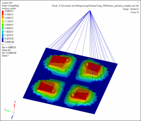
6.	Click Apply. The shape change contour is shown in the window, as follows.

3030_results

Results of random response optimization

Step 7: View the PSD Results in HyperGraph

1.	Launch HyperGraph.

2.	Click the Build Plots icon .

3.	Load the panel_complete.pch file.

4.	The X Type is Frequency (Hz).

5.	Select Group 1 Acceleration as Y Type.

Node id 67 and X_Translation are highlighted.

6.	Click Apply.

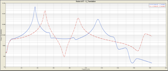
The PSD plot of acceleration in X direction on node 67 at iteration 0 is loaded.

7.	Go to the Axes panel and convert the linear plot of PSD acceleration to logarithmic plot for the y-axis.

8.	Select the last group acceleration as Y Type and repeat steps 6 and 7.

The PSD plot of acceleration in X direction on node 67 at final iteration is loaded.

How much was the peak value of the PSD acceleration reduced?

3030_psd_plots

PSD acceleration plots of the original and the optimized designs.