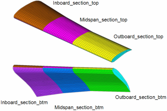
OS-4050: Optimization of a Horizontal Tail Plane

The purpose of this tutorial is to optimize the thickness of the aluminum ribs for a horizontal tail plane (model shown below).

4050_model

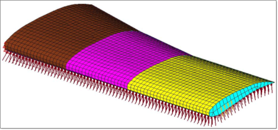
Horizontal tail plane model

It is assumed that the tail is cantilevered about its inboard section. Three loading scenarios are considered; one where the tail experiences pressure loads of 0.25 psi on the bottom skin, a second where the tail experiences a tip load of 400 lbs, and a third where the tail experiences both the pressure load and tip load simultaneously. The applied loading is represented in the following figure.

4050_loading

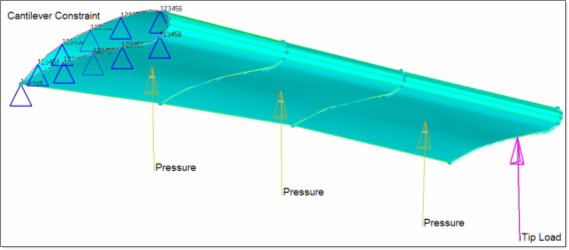
Loading experienced by horizontal tail plane

The materials available for this part are described in the following table. The optimum design should be as light as possible without failing or buckling under the given loading conditions.

	Glass_fabric	Core		Aluminum 2024-T3
E1	4Msi (4.0e6 psi)	2ksi (2000 psi)	E	10.6Msi (10.6e6 psi)
E2	6Msi (6.0e6 psi)	4ksi (4000 psi)	Nu	0.33
NU12	0.1	0.3	G	4.06Msi (4.06e6 psi)
G12	800ksi (800000 psi)	3ksi (3000 psi)	Rho	0.1 lb/in3
G1,Z	800ksi (800000 psi)	4ksi (4000 psi)	Yield	50ksi (50000 psi)
G2,Z	800ksi (800000 psi)	4ksi (4000 psi)
RHO	0.07 lb/in3	0.001074 lb/in3
Xt	35ksi (35000 psi)	500 psi
Xc	35ksi (35000 psi)	500 psi
Yt	35ksi (35000 psi)	500 psi
Yc	35ksi (35000 psi)	500 psi
S	4ksi (4000 psi)	150 psi

The optimization problem may be stated as:

Objective:

Minimize mass.

Constraints:

•	Composite skins must not fail.

•	Aluminum ribs must not yield.

•	Buckling must not occur.

Design variables:

•	Composite ply thicknesses.

•	Rib thicknesses.

In this tutorial, you will learn to:

•	Create material and geometric properties with HyperLaminate

•	Create static and buckling subcases.

•	Perform baseline finite element analysis

•	Run a size optimization and compare results with initial design.

Exercise

Step 1: Launch HyperMesh Desktop, Set the User Profile, and Retrieve the File

1.	Launch HyperMesh Desktop.

2.	Choose OptiStruct in the User Profiles dialog and click OK. This loads the user profile. It includes the appropriate template, macro menu, and import reader, paring down the functionality of HyperMesh to what is relevant for generating models for OptiStruct.

3.	From the File on the main menu, select Open > Model.

4.	Select the tail_baseline.hm file you saved to your working directory from the optistruct.zip file. Refer to Accessing the Model Files.

5.	Click Open.

Step 2: Create Isotropic Materials and Properties and Assign to Metallic Ribs

1.	Click the Model tab on the tab menu to open the Model browser.

2.	In the Model browser, right-click and select Create > Material.

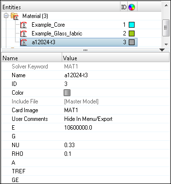
3.	In the Name field, enter al2024-t3.

4.	Set Card Image as MAT1.

5.	Fill in the fields for E, NU and RHO with values 10.6e6, 0.33 and 0.1, respectively.

These values are taken from the table Aluminum 2024-T3 at the beginning of the tutorial.

OS_5040_01

6.	In the Model browser, right-click and select Create > Property.

7.	For Name, enter Ribs.

8.	Set Card Image as PSHELL.

9.	For Material, click Unspecified > Material.

10.	In the Select Material dialog, select a12024-t3 from the list of materials and click OK.

11.	Enter the thickness for the shell component by clicking T and entering 1.0.

12.	In the Model browser, right-click and select Create > Component.

13.	For Name, enter Ribs.

14.	Set the Property to Ribs. This automatically sets the material to a12024-t3.

os_4050_ribs

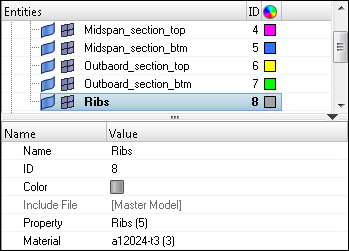
A property collector named Ribs has been created. It has a PSHELL definition with a thickness of 1.0. It also references the Aluminum 2024-T3 material definition and the component name Ribs.

Create Material and Geometric Properties with HyperLaminate

Step 3: Create Orthotropic Material Properties using HyperLaminate

1.	From the 2D page, select the HyperLaminate panel. This launches the HyperLaminate GUI.

2.	On the left-hand tree structure, left click MAT8 to highlight it, and then right-click on the highlighted MAT8. A floating menu appears with one option: New.

3.	Click New.

A new material definition is created and appears in the left-hand tree structure on a branch underneath MAT8.

4.	Under the section Define/Edit material, click in the field to the right of Material:. The default name NewMaterial1 shows.

5.	Replace NewMaterial1 with Glass_fabric.

6.	Fill in the fields for E1, E2, NU12, G12, G1, Z, G2, Z, RHO, Xt, Xc, Yt, Yc, and S with the information provided in the table at the beginning of the tutorial. Refer to the examples in the model, if needed.

7.	Click Apply. An orthotropic material definition for Glass_fabric is now complete.

8.	Repeat steps 3.4 through 3.7 to create other material called Core with the material properties provided in the table. Also select a different color.

You should now have two new orthotropic material definitions on the MAT8 branch of the left-hand tree structure.

Step 4: Create Composite Laminates using HyperLaminate

1.	In the left-hand tree-structure, left-click on PCOMP to highlight it.

2.	Right-click on the pre-highlighted PCOMP. A floating menu appears with one option: New.

3.	Click New.

A new laminate definition is created and appears in the left-hand tree structure on a branch underneath PCOMP.

4.	Under the Laminate definition, replace NewLaminate1 with Inboard_section_top.

5.	To the right of this field, click color and select a color for this laminate.

6.	Under Stacking sequence convention, toggle Convection: to select Symmetric-Midlayer.

7.	Under Add/Update plies, make the following selections/assignments:

- For Material, select Glass_fabric.

- For Thickness T1, enter 0.25.

- For Orientation (Degrees), enter 0.

- For No. of Repetitions, enter 1.

8.	Click Add new ply three times.

9.	Under Ply lay-up order, in the 2nd row, modify the information:

- For Material, select Core.

- For Thickness T1, enter 0.5.

- For Orientation (Degrees), enter 45.

10.	Under Ply lay-up order, in the 1st row, modify the information:

- For Orientation (Degrees), enter 90.

The Ply lay-up order should appear like the image below.

4050_plylayup

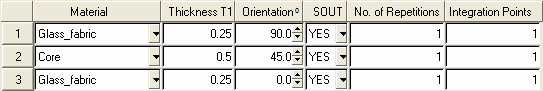
Ply lay-up order for inboard_section_top.

11.	Click Update Laminate.

The definition of the Inboard_section_top laminate is now complete. The following figure shows the laminate as displayed in the right-hand side Review panel.

4050_update_lam

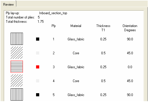
Inboard_section Laminate

12.	Right-click on Inboard_section_top and select Duplicate.

13.	Rename the PCOMP to Inboard_section_btm by right-clicking on the PCOMP or editing the Name: field and changing the color.

14.	Update the ply angles on the other four laminates (Outboard_section_btm, Outboard_section_top, Midspan_section_btm, and Midspan_section_top) to be the same as shown previously.

15.	Click Update Laminate.

You should now have six laminate definitions on the PCOMP branch of the left-hand tree structure. The tree-structure should look like the one shown in the figure below at this point.

os_4050_002

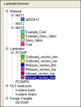
HyperLaminate tree structure showing one isotropic material, four anisotropic materials, and six laminate definitions

16.	From the File menu, select Exit.

This will let you exit the HyperLaminate GUI, and will export the information back to HyperMesh.

Step 5: Assign Newly Created Properties to the Associated Component

At this point, the model is meshed and the material and geometric properties are defined. However, the elements are not referencing the correct property and material information.

1.	Expand the Component branch of the Model browser tree. Right-click on the Inboard_section_top collector and select Assign.

2.	Select the property Inboard_section_top from the list in the dialog box and click OK to return to the main window.

3.	Repeat this process to assign the Inboard_section_btm property to the Inboard_section_btm collector.

Step 6: Organize Elements into their Respective Component Collectors

1.	In the Model browser, right-click on LoadCollector, and select Hide.

2.	Press the letter o on the keyboard (for the Options panel).

3.	Set the mesh radio button on the left hand side of the panel.

4.	Set the feature angle= to 37. This allows you to select elements by feature angle.

5.	Click return.

6.	From Tool page, select the organize panel.

7.	Select one of the elements on the top inboard section, shown in brown in the picture below.

8.	Click elems and select by face.

Notice a number of elements are selected on the top surface, stopping where the angle between elements is greater than 37 degrees. The ribs elements in between the top and bottom surface create a 90 degrees, thus the selection set stops here.

9.	Click dest = and select Inboard_section_top from the list of component collectors.

10.	Click Move.

11.	Repeat steps 6.7 through 6.9 to generate a similar picture below.

4050_skin_elements

Skin elements organized into correct component collectors.

12.	Right-click on Tail and select Isolate Only. Only the elements forming the ribs which are in the tail collector should now be displayed.

13.	From Tool page, select the organize panel.

14.	Click elems and select displayed.

15.	Click Destination = and select Ribs from the list of component collectors.

16.	Click Move.

17.	In the Model browser, right-click on Component and select Show.

18.	Click return to return to the main menu.

19.	Press F2 on the keyboard.

20.	Set the entity selection to comps.

21.	Click preview empty and delete entity to clear any empty components (the tail component in this case).

22.	Click Return.

Step 7: Orient Elements Which Reference Composite Properties

1.	From Tool page, select the normals panel.

2.	Make sure the elements radio button is selected at the left of the panel.

3.	Set the entity selection type to elems.

4.	Click elems and select by collector.

5.	Check the box next to Ribs.

6.	Click the comps entity selection and select reverse from the extended selection list.

7.	Click select.

8.	Click display normals.

You may verify if the element normals are not all in the same direction. If they are not, follow steps 9 and 10.

9.	Click elem under orientation: and select an element whose normal is pointing inward.

10.	Click adjust normals.

All "skin" normals should now point inwards. These skin normals are the local z-axes for each element.

11.	Click return to return to the main menu.

12.	From the 2D page, select the composites panel.

13.	Make sure the radio button is set to material orientation.

14.	Select those elements belonging to the "skin" (all the comps except ribs) components.

15.	Click the switch under Material orientation method: and select by vector from the drop-down menu.

16.	Click on the switch under by vector and select z-axis from the drop-down menu.

17.	Click project.

This orients the local x-axis of each of the selected elements to be the projection of the global z-axis. This is displayed graphically by the small white arrows that appear on each element.

Having defined the local x and z axes of the elements belonging to the component collectors Inboard_section_top, Inboard_section_btm, Midspan_section_top, Midspan_section_btm, Outboard_section_top, and Outboard_section_btm, you have fully established the local orientation for each element referencing a composite laminate.

18.	Click return.

Create Static and Buckling Subcases

Three loading scenarios are to be considered in this exercise: one where the tail experiences pressure loads on the bottom skin, a second where the tail experiences a tip load, and a third where the tail experiences both the pressure load and tip load simultaneously.

In previous steps, a load collector containing the pressure loads and another containing the tip load were created, but a load collector containing both together is still needed. Next is to create a load collector which is a combination of the load collectors pressure and tip_load.

Step 8: Create a Combination Load Collector

1.	In the Model browser, right-click and select Create > Load Collector.

2.	In the Name field, enter Combined.

3.	Select a suitable color.

4.	Set Card Image to LOAD. For information on the LOAD card, refer to the OptiStruct online help.

5.	Click S and enter 1.0.

6.	Click LOAD_Num_Set = and enter 2. This indicates how many load-collectors to combine.

7.	In the pop-out window, enter S1(1) = 1.0, for L1(1), select pressure from the list of load collectors, enter S1(2) = 1.0 and for L1(2), select tip_load from the list of load collectors.

8.	Click Close.

A combination load collector, combining 1.0 times the loads in the pressure load-collector with 1.0 times the loads in the tip_load collector, is created.

Step 9: Create a Static and Associated Buckling Subcase

1.	Click View > Browsers > HyperMesh > Utility to open the Utility tab.

2.	In the Utility tab, select FEA.

3.	Under Loadsteps:, click Buckling. The Create Buckling Subcases window appears.

With this window, a static subcase and an associated buckling subcase in one step will be created.

4.	For Name:, enter pressure_only. This is the user-defined name for the static subcase.

If you call the static subcase name, then the associated buckling subcase will be named buck_name.

5.	Select EIGRL from the drop-down menu that follows the field for Name:. This indicates that eigenvalue analysis is to be used to calculate the buckling modes. Currently this is the only option available.

6.	In the field for V1:, enter 0.0.

This indicates that the lower bound for the eigenvalue extraction is 0.0. This prevents negative buckling modes being calculated (negative buckling modes indicate that buckling will occur if the loading is reversed).

7.	The field for V2: may be left blank.

This is the upper bound for the eigenvalue extraction. You will select a number of modes to calculate (instead of a range of eigenvalues) for this exercise.

8.	In the field for ND:, enter 10.

This requests that the 10 lowest buckling modes (which are greater than V1) be calculated.

9.	Select pressure from the drop-down list to the right of LOAD:.

10.	Select constraints from the drop-down list to the right of SPC:.

11.	Click Create.

You have now created a linear static subcase named pressure_only which combines the pressure loads in the load-collector pressure with the single-point constraints in the load collector constraints.

An associated buckling eigenvalue subcase named buck_pressure_only is also created which will calculate the first 10 buckling modes greater than 0.0 for the pressure_only static subcase.

12.	Repeat steps 3 through 11 to create a static subcase named tip_load_only, which combines the point loads in the load-collector tip_load with the single point constraints in the load collector constraints, and an associated buckling subcase which will calculate the first 10 modes greater than 0.0.

13.

Repeat steps 3 through 11 again to create a static subcase named combo, which combines the loads in the load-collector combined (i.e. both pressure and tip_load) with the single point constraints in the load collector constraints, and an associated buckling subcase which will calculate the first 10 modes greater than 0.0.

14.	Close the Create Buckling Subcases window.

Step 10: Request Stress, Strain, and Failure Results for Composite Laminates

Stress, strain, and failure results are not output by default for composite laminates, but need to be requested.

1.	In the Model browser, right-click on the Outboard_section_top property and select Card Edit.

The PCOMP card image for the Outboard_section_top laminate appears in the lower portion of the display area. For more details on the PCOMP card image, refer to the OptiStruct online documentation.

2.	If HILL does not appear beneath [FT], click [FT] notice HILL appears beneath.

This activates failure theory calculation. If HILL is selected, a list of other failure theories appear - use the Hill failure criteria for this exercise.

3.	Click [SB] in the card image window and enter 3,500 in the field beneath it.

This is the interlaminate shear strength of the laminate, which is the bonding material shear strength. 3.5ksi is an assumed value, as no material data was provided.

4.	Click the button beneath SOUT(1) and select YES from the pop-up menu. This requests stress and strain results to be output for ply1.

5.	Set all other plies, i.e. SOUT(2), SOUT(3), SOUT(4) and SOUT(5) to YES also.

6.	Click return to keep the changes you made to the card image.

7.	Repeat steps 3 through 9 for the other composite laminates.

Note:

Select all PCOMP props in step 3 to reduce steps. Make sure HILL is selected.

8.	Click return to return to the main menu.

9.	From Analysis page, select the control cards panel, and enter GLOBAL_CASE_REQUEST.

10.	Make sure CSTRAIN is selected from the list of control cards. The CSTRAIN card image appears in the lower portion of the display area.

11.	Make sure CSTRESS is selected from the list of control cards. The CSTRESS card image appears in the lower portion of the display area.

Stress, strain, and failure results will now be output for the composite laminates.

12.	Click return until you return to the main menu.

Step 11: Perform the Baseline Finite Element Analysis

1.	From the Analysis page, enter the OptiStruct panel.

2.	Click save as, enter tail_baseline_complete.fem as the file name, and click Save.

3.	Set export options: to all.

4.	Set run options: to analysis.

5.	Set memory options: to memory default.

6.	Leave the options: field blank.

7.	Click OptiStruct to run the analysis job.

The message Processing complete appears in the window at the completion of the job. OptiStruct also reports error messages if any exist. The file tail_baseline_complete.out can be opened in a text editor to find details regarding any errors. This file is written to the same directory as the .fem file.

8.	Close the DOS window or shell and click return.

Step 12: Review the .out Analysis Summary File

In the directory where you ran the OptiStruct analysis, you should find a tail_baseline_complete.out file. This file contains a summary of the analysis run.

Using a text editor of you choice, open the file tail_baseline_complete.out.

The file contains:

•	A summary of the finite element model.

•	A summary of the optimization parameters.

•	Memory and disk space estimations.

•	Analysis results.

The Volume, Mass, and Buckling Modes for the baseline model are given in the analysis results section, as shown in the following tail_baseline_complete.out analysis results section:

ANALYSIS RESULTS :

------------------

ITERATION 0

(Scratch disk space usage for starting iteration = 30 MB)

(Running in-core solution)

Volume = 7.71079E+04 Mass = 2.49519E+03

Subcase Compliance

1 5.455666E+02

3 2.486638E+01

5 7.735856E+02

Subcase Mode Buckling Eigenvalue

2 1 1.583435E+01

2 2 1.610702E+01

2 3 1.638024E+01

2 4 1.665444E+01

2 5 1.681097E+01

2 6 1.693918E+01

2 7 1.715172E+01

2 8 1.723870E+01

2 9 1.739906E+01

2 10 1.748200E+01

4 1 8.267695E+01

4 2 8.326373E+01

4 3 8.393269E+01

4 4 8.466939E+01

4 5 8.541136E+01

4 6 8.618942E+01

4 7 8.695226E+01

4 8 8.765920E+01

4 9 8.834313E+01

4 10 8.907416E+01

6 1 1.329775E+01

6 2 1.351079E+01

6 3 1.372538E+01

6 4 1.394187E+01

6 5 1.416444E+01

6 6 1.417737E+01

6 7 1.439755E+01

6 8 1.445274E+01

6 9 1.464175E+01

6 10 1.466889E+01

Step 13: Review the Displacement Results

1.	When the message Process completed successfully is received in the command window, click HyperView. HyperView is launched and the results are loaded.

A message window appears to inform about the successful loading of the model and result files into the HyperView client in a new page.

2.	Click Close to close the message window.

3.	Set the animation type to Linear .

4.	Click the Contour toolbar icon .

5.	Make sure that the Result type: is Displacement [v]. The second drop-down menu shows Mag.

6.	Click Apply to display the displacement contour.

Note that this capture is shown for the 1st subcase [pressure only]. You could also view the same for other subcases.

4040_displacement_contour

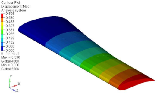
Displacement contour for pressure_only subcase.

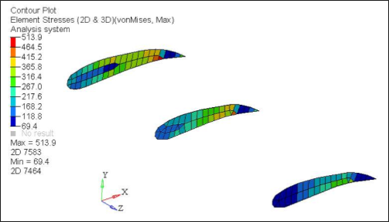
Step 14: Review the Stress Results in HyperView

1.	Click the Entity Attributes toolbar icon .

2.	Make sure that the box for Auto apply mode: is checked.

3.	Click Off to the right of Display:. This will cause any component selected, either in the display or from the list of components, to be hidden.

4.	Hide all of the components except the ribs by clicking them in the GUI.

5.	Click the Contour toolbar icon or select Contour from the Graphics menu.

6.	Toggle the Result type: to Element Stresses (2D & 3D) [t].

7.	Make sure the second drop-down menu shows von Mises.

8.	Click Apply. This shows a contour plot of the von Mises stresses for the metallic ribs.

os_4050_contour_plot

9.	Click the Entity Attributes toolbar icon.

10.	Click Flip. The Ribs component is now hidden and the composite laminate components are displayed.

11.	Click the Contour toolbar icon or select Contour from the Graphics menu.

12.	Set Result type: to Composite Stresses (s) from the first row and Ply Failure from the second row.

13.	On the third list, select Entity with Layers: 1.

14.	Click Apply.

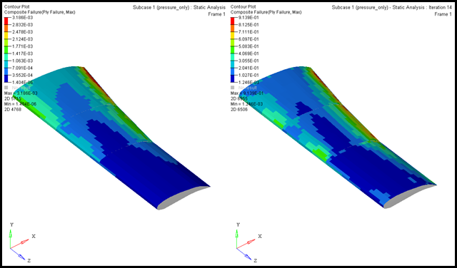
A contour plot of the composite failure indices from the composite skins results is displayed for the first layer.

os_4050_fail_index

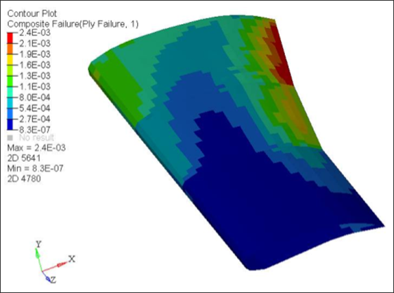
Failure index for the first layer for the pressure only loadstep.

After calculating the failure indices for individual plies, OptiStruct calculates the potential failure index for the composite shell element. This is based on the premise that failure of a single layer qualifies as failure of the composite. Thus, a failure index for composite elements is calculated as a maximum of all computed ply and bonding failure indices (note that only plies with requested stress output are taken into account here).

15.	Change Entity with Layers: to Max to have the maximum index for the laminate.

os_4050_max_fail

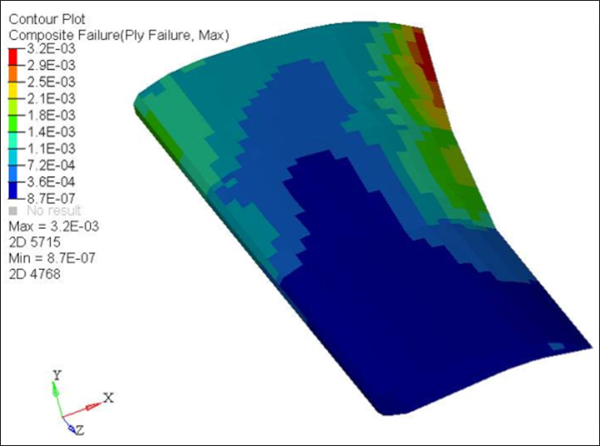
Max failure index found on all layers for pressure only loadstep.

Repeat this process to have the maximum failure index for all loadsteps.

MAX FAILURE INDEX = 3.73 e-3 (Combo Loadstep)

Run a Size Optimization and Compare Results with Initial Design

Now return to HyperMesh to set up the optimization problem. The first step in this process is to define the design variables. The design variables for this exercise are the rib thicknesses and the laminates used in the composite skins.

HyperMesh Desktop allows you to use one HyperMesh page and multiple pages from the HyperView, HyperGraph, MotionView, and MediaView clients without having to switch applications. To delete the HyperView page and return to the HyperMesh client, click the Delete Page icon . To keep the page open but return to the HyperMesh client page, click the Previous Page or Next Page icons until the HyperMesh client returns.

Step 15: Create and Reference a Thickness Design Variable for the Metallic Ribs

1.	From Analysis page, select the optimization panel.

2.	From optimization panel, select the gauge panel.

3.	Make sure the radio button is set to create.

4.	Click props and select the Ribs collector.

5.	Make sure that the top toggle is set to value from property. This sets the initial value of the design variable to be the thickness value defined on the property card.

6.	Toggle lower bound % to lower bound = and enter 0.01. This sets the lower bound for the design variable.

7.	Toggle upper bound % to upper bound = and enter 2.0. This sets the upper bound for the design variable.

8.	Make sure type: is set to PSHELL - T.

The following figure shows how the settings should look.

os_4050_settings

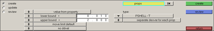
Gauge panel settings for rib thickness design variable

9.	Click create.

10.	Click return twice to go to the main page.

Step 16: Create Design Variables for Composite Laminates with HyperLaminate

1.	From the 2D page, select the HyperLaminate panel. This launches the HyperLaminate GUI.

2.	In the tree-structure on the left, click DESVAR to highlight it.

3.	Right-click on the pre-highlighted DESVAR. A menu appears with options.

4.	Select New. This creates a new design variable, which is named NewDv1 by default.

5.	Rename the design variable istgf_th (inboard_section_top, glass_fabric, and thickness) by double-clicking in the text field following Desvar: and overwriting the default design variable name.

6.	In the Initial Value: field, enter 0.25.

7.	In the Lower Bound: field, enter 0.01.

8.	in the Upper Bound: field, enter 1.0.

9.	Click Apply.

10.	In a similar manner, and with identical values, create one more design variables named isbgf_th following the procedure outlined in steps 4 through 9.

Alternately, right-click on istgf_th and select Duplicate from the menu to create an identical design variable. Repeat this process to create the other design variables, then rename the new design variables by right-clicking on them and selecting Rename.

11.	Review the other ten design variables in HyperLaminate and the information in the table below.

Name	Initial Value	Lower bound	Upper bound
mstgf_th	0.25	0.01	1.0
msbgf_th	0.25	0.01	1.0
ostgf_th	0.25	0.01	1.0
osbgf_th	0.25	0.01	1.0
istc_th	0.5	0.01	2.0
isbc_th	0.5	0.01	2.0
mstc_th	0.5	0.01	2.0
msbc_th	0.5	0.01	2.0
ostc_th	0.5	0.01	2.0
osbc_th	0.5	0.01	2.0

Twelve total composite design variables now exist, one for the thickness of the glass fabric for each composite laminate component, and the other for the thickness of the core for each composite laminate component. As the laminates are symmetric, the glass fabric will reference the same design variables on either side of the core.

Step 17: Update Composite Laminate Properties as Design Variables using HyperLaminate

1.	Click Inboard_section_top under the PCOMP branch of the tree-structure. Details of the laminate appear in the GUI.

2.	Click the checkbox next to Optimization. New fields appear in the Entry Rows table, allowing design variables to be associated to ply thicknesses or ply orientations.

3.	Under Ply lay-up order, click on the field under Designvar, under Thickness in row 1.

4.	Select istgf_th from the drop-down menu.

Now the design variable istgf_th is associated to the thickness of the Glass_fabric material used in ply1, and, in this case, ply5 (as this is a symmetric-midlayer type laminate) of the Inboard_section_top component collector.

5.	Click in the field under Designvar, under Thickness in row 2.

6.	Select istc_th from the drop-down menu.

Now the design variable istc_th is associated to the thickness of the Core material used in ply2 and ply4 of the Inboard_section_top component collector.

7.	Click in the field under Designvar, under Thickness in row 3.

8.	Select istgf_th from the drop-down menu.

9.	Click Update Laminate to save the design variable assignments.

10.	Repeat steps 1 through 9 for Inboard_section_btm composite laminate component collector, associating the appropriate design variables.

11.	From the File menu, select Exit.

This will close the HyperLaminate GUI, exporting the design variable and updated laminate information back to HyperMesh.

Step 18: Create the Mass, Static Stress and Composite Failure Responses

1.	From the Analysis page, select the optimization panel.

2.	Select responses.

3.	Click response= and enter mass.

4.	Click the response type: switch and select mass from the pop-up menu.

5.	Click create. The optimization response mass, which is the total mass of the structure, is created.

6.	Click response= and enter vm_strs.

7.	Click the response type: switch and select static stress from the pop-up menu.

8.	Click props and select the Ribs collector.

9.	Click Select. A new selector switch appears next to comps.

10.	Make sure that the switch is set to von Mises.

11.	Click the switch below von Mises and set it to both surfaces.

12.	Click create. The optimization response vm_strs, which is the von Mises stress for the metallic ribs, is created.

13.	Click response= and enter hl_ist.

14.	Click the response type: switch and select composite failure from the pop-up menu.

15.	Click props and select the Inboard_section_top collector.

16.	Click the switch next to props and select hill.

17.	Click the switch below hill and select all plies.

18.	Click create. The optimization response hl_ist is created.

This is the hill failure criteria for all plies of the composite skins of the Inboard_section_top component collector.

19.	Repeat steps 12 through 18 to create optimization responses for the hill failure criteria for the plies of the other composite laminate skins. The responses could be similarly named: hl_osb, hl_ost, hl_msb, hl_mst, and hl_isb.

20.	Click response= and enter buckle.

21.	Click the response type: switch and select buckling from the pop-up menu.

22.	Click Mode Number: and enter 1.

23.	Click create. The optimization response buckle, which is the lowest calculated buckling mode for the structure, is created.

24.	Click return to return to the optimization panel.

Step 19: Create Constraints and an Objective

Finally, the constraints and objectives must be defined. You will attempt to minimize the total mass of the structure, while keeping the von Mises stress in the metallic ribs below yield, the composite failure index of the composite skins below 1.0, and the buckling modes of the structure above 1.0.

1.	Select the dconstraints panel.

2.	Click constraints = and enter cnst1.

3.	Click response = and select vm_strs.

4.	Check the box preceding upper bound =.

5.	Click upper bound = and enter 50,000.

6.	Click loadsteps and select the loadsteps pressure_only, tip_load_only, and combo.

7.	Click select.

8.	Click create. This defines a constraint on the von Mises stress of the metallic ribs to be less than 50ksi for all of the static subcases.

9.	Click constraints = and enter cnst2.

10.	Click response = and select hl_ist.

11.	Check the box preceding upper bound =.

12.	Click upper bound = and enter 1.0.

13.	Click loadsteps and select the loadsteps pressure_only, tip_load_only and combo.

14.	Click select.

15.	Click create. This defines a constraint on the hill failure criteria for the Inboard_section_top laminate to be less than 1.0. for all of the static subcases.

16.	Repeat steps 9 through 15 for all the other failure criteria responses, creating cnst3 through cnst7.

17.	Click constraints = and enter cnst8.

18.	Click response = and select buckle.

19.	Uncheck the box preceding upper bound =.

20.	Check the box preceding lower bound =.

21.	Click lower bound = and enter 1.0.

22.	Click loadsteps and select the loadsteps buck_pressure_only, buck_tip_load_only and buck_combo.

23.	Click select.

24.	Click create. This defines a constraint on the lowest calculated buckling mode of the structure to be greater than 1.0 for all of the linear buckling subcases.

25.	Click return to return to the optimization panel.

26.	Select the objective panel.

27.	Click the left-hand switch and select min.

28.	Click response = and select mass from the pop-up menu.

29.	Click create. This defines the objective of the optimization to minimize the mass of the structure.

30.	Click return to return to the optimization panel.

Step 20: Create Additional Run Parameters to Aid Buckling Constraints

For the buckling constraint to be effectively maintained, an additional parameter needs to be defined.

1.	Select the opti control panel.

2.	Check the box preceding MAXBUCK=. The box preceding GBUCK= is checked automatically.

Together, these two options ensure that up to 10 modes are considered in the buckling constraint. Refer to the OptiStruct online help for a more detailed description.

3.	Click return.

Step 21: Run the Optimization Problem

1.	From the Analysis page, enter the OptiStruct panel.

2.	Click save as, enter tail_opt.fem as the file name, and click Save.

3.	Set the export options: toggle to all.

4.	Set the run options: toggle to optimization.

5.	Set the memory options: toggle to memory default.

6.	Click OptiStruct.

The message Processing complete appears in the window at the completion of the job. OptiStruct also reports error messages if any exist. The file tail_opt.fem.out can be opened in a text editor to find details regarding any errors. This file is written to the same directory as the .fem file.

7.	Close the DOS window or shell and click return.

Step 22: Review the .out Optimization Summary File

In the directory where you ran the OptiStruct optimization, you should find a tail_opt.out file. This file contains a summary of the optimization run.

Using a text editor of your choice, open the file tail_opt.out.

The file contains:

•	A summary of the finite element model.

•	A summary of the optimization parameters.

•	Memory and disk space estimations.

•	An optimization iteration history.

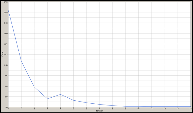
The value of the objective, the retained constraints, and the design variables are provided for all iterations in the optimization iteration history section. The sample output for the final iteration is shown in the plot of objective against iteration below.

The final iteration provides information on the mass of the optimized structure, the values of the design variables for the optimized structure and the values of the objective and retained constraints for the optimized structure.

Step 23: Review the Iteration History in HyperView

In addition to looking at the information in the tail_opt.out file, graphically review the iteration history of the optimization using HyperView.

1.	Create a new page with the HyperView client by using the Add Page icon .

2.	From the File menu, select Open > Session. The Open Session File window appears.

3.	Select the file tail_opt_hist.mvw from the directory where you ran the OptiStruct optimization.

This is a HyperView session which creates plots of the objective, constraints, and design variables against iteration number using information from the tail_opt.hist file.

The figure below shows page 1 of the session, which is the plot of the objective against iteration. It shows how the mass decreased through the optimization process and how convergence is achieved when the change in mass levels out.

Similar plots are available for the design variables and the constraints. There is also a plot showing the maximum constraint violation for a given iteration against iteration. When this value is zero, it indicates that there is no constraint violation.

os_4050_obj_function

Step 24: Compare the Baseline Results with Optimized Results in HyperView

1.	Click File > New > Session to start a new session.

2.	Change the current client to HyperView using the client selector drop-down .

3.	Click the down arrow to the right of the Select application toolbar icon and select HyperView .

4.	Click Yes to continue.

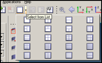
5.	Create a two pane view by clicking on the Page Window Layout icon and selecting the two view icon from the pop-up menu.

os_4050_page_layout

6.	Activate the left-hand pane by clicking anywhere in it. The active pane is the one surrounded by the blue halo.

7.	Click the Load results toolbar icon . The Load Model File panel opens.

8.	Select the Tail_baseline_complete.h3d file from the directory where you ran your OptiStruct baseline analysis.

9.	Click Open.

The path and file name for Tail_baseline_complete.h3d appears in the fields to the right of Load model and Load results. This is good because the Hyper3D format contains both model and results data.

10.	Click Apply. The model and results are loaded in the current HyperView window.

11.	Activate the right-hand window by clicking on it.

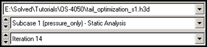
12.	Repeat steps 5 through 8 to load the file tail_opt_s1.h3d from the directory where you ran your OptiStruct optimization.

For the optimization, analysis results are written to files named *_s#.h3d (static analysis results, where # is the subcase ID) and *_m#.h3d (eigenvalue analysis results, where # is the subcase number), while the density, thickness and shape results are written to the file *_des.h3d.

13.	Activate the left-hand pane by clicking on it.

14.	Click the Contour toolbar icon .

15.	Select Displacement (v) from the drop-down menu under Result type:.

16.	Click Apply.

17.	Activate the right-hand pane.

18.	In the Load Case Simulation Selection window above the Results browser, select subcase 1 (pressure only) in the Load Case area and select the last ITER # in the Simulation area.

os_4050_subcase1

19.

Click OK.

20.	Click the Contour toolbar icon .

21.	Select Displacement (v) from the drop-down menu under Result type:.

22.	Click Apply.

Now visible is a side-by-side comparison of the displacement results before the optimization with those after the optimization (figure below); note the big change in the value of the total displacement. The optimized displacement results are greater than the baseline because you were optimizing for mass without displacement constraints.

os_4050_base_optimize

23.	With the animation mode set to Linear static , click the Play icon to animate the deformation.

24.	Click again to stop the animation.

Similar steps can be followed to compare stress and composite failure plots before and after the optimization.

Notice how the maximum value for the composite failure index is almost at the design limit of 1.0.

Assigning Thicknesses and Orientations

Step 25: Import the Optimum Property Information into HyperMesh

1.	From the File menu, select New > Session.

2.	Set the Client Selector drop-down to the HyperMesh client .

This clears all results information out of the client, including all pages. This will not affect your files on your hard drive.

3.	From the File menu, click Import > Solver Deck.

4.	Click the file folder icon at the end of the File: field and select the tail_opt.fem file from the directory where you ran the optimization.

5.	Click Import. This loads the *.fem that the optimization was run with into HyperMesh.

6.	Click the file folder icon at the end of the File: field and select the tail_opt.prop file from the directory where you ran the optimization.

The tail_opt.prop file is created by OptiStruct at the end of the optimization run and contains the optimized property data for model.

7.	In the Import tab, click the arrow before the import options to expand.

8.	Check the box beside FE overwrite.

9.	Click Import.

10.	From the 2D page, select the HyperLaminate panel.

11.	Click through the PCOMP properties and review the new thickness.

Conclusion

The objective of this tutorial was to achieve the lightest design by varying the laminate properties and rib thicknesses. Experimenting with other materials and other laminate configurations could lead to a lighter design.