OS-4070: Free-sizing Nonlinear Gap Optimization on an Airplane Wing Rib

In this tutorial, an existing finite element model of an aluminum wing rib model is used to demonstrate how to do free-sizing optimization using OptiStruct. HyperView is used to post-process the thickness pattern in the rib.

os4070_pic1

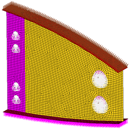
Wing rib model

There are four shell components in the model: the mounting flange, the web, the top and bottom flanges, and the lug. The web is connected to the lug by gap elements. Appropriate properties, loads, boundary conditions, and nonlinear subcases have already been defined in the model. The design region is the web and the rest of the components are non-design. Since a large portion of aerospace components are shell structures which are manufactured by machining or milling operations, free-sizing optimization is very suitable for those components. To understand the limitations of topology optimization for such applications, a nonlinear gap topology optimization will also be done on the wing rib model.

The optimization problem for this tutorial is stated as:

Objective:	Minimize weighted compliance WCOMP.
Constraints:	Volume fraction on the web < 0.3.
Design variables for free sizing optimization:	Thickness of each shell element in the design space.
Design variables for topology optimization:	Element density of each element in the design domain.

In this tutorial, you will learn to:

•	Setup a free-sizing optimization with nonlinear gap elements

•	Post-process the thickness convergence in the design domain

•	Setup a topology optimization with nonlinear gap elements

•	Post-process the material distribution in the design domain

•	Review and compare results from free-size optimization and topology optimization

Exercise

Step 1: Launch HyperMesh Desktop, Set the User Profile, and Retrieve the File

1.	Launch HyperMesh Desktop.

2.	Choose OptiStruct in the User Profiles dialog and click OK.

3.	From the File menu on the toolbar, select Open Model. An Open Model browser window opens.

4.	Select the rib_complete.hm file you saved to your working directory from the optistruct.zip file. Refer to Accessing the Model Files.

5.	Click Open.

Step 2: Create Design Variable for Free-sizing Optimization

1.	From the Analysis page, select the optimization panel.

2.	Select the free size panel.

3.	Choose the create subpanel using the radio button on the left.

4.	Click desvar= and enter shells.

5.	Verify that type: is set to PSHELL.

6.	Click props, choose the Web component and click select.

7.	Click create. This creates the design variable for free-sizing optimization.

Step 3: Create Manufacturing Constraints for Free-sizing

1.	While still in the Free Size Optimization panel, select the parameters subpanel.

2.	Click desvars and select the shells design variable created previously.

3.	Toggle minmemb off and, for mindim =, enter 2.0.

4.	Click update.

5.	Click return.

Step 4: Create Optimization Responses, Objective, and Constraints

1.	Select the responses panel.

First, the weighted compliance response will be created.

2.	For response =, input the name wcomp.

3.	Click the switch for response type and click weighted comp.

4.	Click loadsteps and select both the Coup_Ver and Pressure loadcases. The weighting factor should be 1.0 for both.

5.	Click return.

6.	Click create.

7.	For response =, input the name volfrac to create the volume fraction response.

8.	For response type, click volume frac.

9.	Leave the type as total.

10.	Click create.

11.	Click return.

12.	Click the dconstraints panel to define the volume fraction constraint.

13.	For constraint =, input the name vol.

14.	Click response =, and select the volfrac response.

15.	For upper bound =, input a value of 0.3.

16.	Click create.

17.	Click return.

18.	Click the objective panel to define the objective.

19.	Toggle to min if not already done.

20.	For response =, select the wcomp response.

21.	Click create.

22.	Click return twice to exit the panel. The optimization parameters have now been defined.

Step 5: Run Free-sizing Nonlinear Gap Optimization

1.	From the Analysis page, select the OptiStruct panel.

2.	Click save as following the input file: field.

3.	Select the directory where you would like to write the optimization file and enter the name rib_freesize.fem in the File name: field.

4.	Click Save.

The name and location of the rib_freesize.fem file displays in the input file: field.

5.	Set the export options: toggle to all.

6.	Set the run options: toggle to optimization.

7.	Set the memory options: toggle to memory default.

8.	Click OptiStruct. This launches the OptiStruct job.

If the job was successful, new results files can be seen in the directory where the OptiStruct model file was written. The rib_freesize.out file is a good place to look for error messages that will help to debug the input deck if any errors are present.

The default files written to the directory are:

rib_freesize.hgdata	HyperGraph file containing data for the objective function, percent constraint violations, and constraint for each iteration.
rib_freesize_hist.mvw	This file is a HypeView session file and may be opened from the File menu in HyperView or HyperGraph. The file automatically creates individual plots for each of the results (objectives, constraints) contained in the .hist file. Each plot occupies its own page within HyperView (HyperGraph).
rib_freesize.HM.comp.cmf	This is a HyperMesh command file. When executed in HyperMesh, the .HM.comp.cmf file organizes all elements in the model into ten new components based on their element thicknesses at the final iteration. The components for this run are named 0.0-0.01, 0.01-0.02, 0.02-0.03, and so on, up to 0.09-0.1, considering the plate thickness of the Web is 0.1mm.
rib_freesize.HM.ent.cmf	This is a HyperMesh command file. When executed in HyperMesh, the .HM.ent.cmf file organizes all elements in the model into ten new sets based on their element thicknesses at the final iteration. The set for this run are named 0.0-0.01, 0.01-0.02, 0.02-0.03, and so on, up to 0.09-0.1, considering the plate thickness of the Web is 0.1mm.
rib_freesize.html	HTML report of the optimization, giving a summary of the problem formulation and the results from the final iteration.
rib_freesize_frame.html	The file contains two frames. The top frame opens one of the .h3d files using the HyperView Player browser plug-in. The .h3d file opened depends on the results selected for display in the bottom frame. The bottom frame opens the _menu.html file, which facilitates the selection of results to be displayed.
rib_freesize_menu.html	This file facilitates the selection of the appropriate .h3d file for the HyperView Player browser plug-in in the top frame of the _frames.html file, based on chosen results.
rib_freesize.oss	The file contains default settings for running OSSmooth after a successful optimization.
rib_freesize.out	OptiStruct output file containing specific information on the file setup, the setup of the optimization problem, estimates for the amount of RAM and disk space required for the run, information for all optimization iterations, and compute time information. Review this file for warnings and errors that are flagged from processing the rib_freesize.fem file.
rib_freesize.res	HyperMesh binary results file.
rib_freesize.sh	Shape file for the final iteration. The .sh file may be used to restart a run.
rib_freesize.stat	Summary of analysis process, providing CPU information for each step during analysis process.
rib_freesize_des.h3d	HyperView binary results file for element thickness information.
rib_freesize_s1.h3d	HyperView binary results file for displacement and stress results for subcase 1.
rib_freesize_s2.h3d	HyperView binary results file for displacement and stress results for subcase 2.
rib_freesize.fsthick	The element definitions for those elements that were part of a free size design space. The optimized thickness of these elements is provided as nodal thickness values (Ti).
rib_freesize.hist	ASCII table file with: Iteration Objective Max_Const_Violation Design_variables DRESP1s DESP2s.
rib_freesize.mvw	This file is a HypeView session file and may be opened from the File menu in HyperView. The file automatically creates individual load the optimization results (dens.h3d) and the loadstep results (s#.h3d).

Post-process the Thickness Convergence in the Design Domain

Element thickness distributions are output from OptiStruct for all iterations. In addition, Displacement and Stress results are output for each subcase for the first and last iteration by default. This section describes how to view those results in HyperView.

1.	From the OptiStruct panel, click HyperView.

This should open a new window with the HyperView client and load the rib_freesize.h3d, reading the model and the results.

2.	Click close to close the message window.

3.	Click the Entity Attributes icon on the toolbar and undisplay all of the components, except Web. This is accomplished by activating the Auto apply mode: (Display OFF) and then clicking on the component that you want turned off in the GUI.

4.	Click the Mesh:, shaded mesh option .

5.	Click the Web component to get a shaded mesh.

6.	Go to the Contour panel and set the Result type: to Element Thicknesses.

7.	In the loadcase selection area above the Results browser, select the last iteration listed in the Simulation list and click OK.

os4070_iteration

8.	Click Top View to get a top view of the Web.

This will show the contour element thickness on the Web component.

4070_thickness_contour

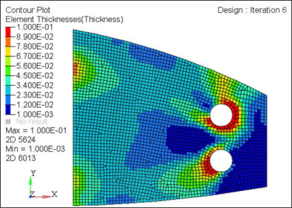
Thickness contour from free-sizing nonlinear gap optimization, on the Web of plate thickness 0.1mm

As can be seen from the figure above, the result from free-sizing optimization is a web with optimized thickness distribution that can be reduced subsequently into larger zones for simplification of the manufacturing process. Moreover, the design obtained from free-sizing offers the freedom to create cavities, ribs, and varying thickness simultaneously, which is not possible in topology optimization.

9.	Close the HyperView client pages by clicking Delete Page until the HyperMesh client is on screen again.

Setting Up a Topology Optimization with Nonlinear Gap Elements

Step 6: Create Design Variables for Topology Optimization

1.	First, save the current HyperMesh file by selecting the File menu and clicking Save as > Model.

2.	Select the directory where you are running the optimization and enter rib_freesize.hm for the file name.

3.	Click save.

4.	Right-click on the Design Variable section of the Model browser and select Delete.

5.	From the Analysis page, select the optimization panel.

6.	Choose the topology panel.

7.	Select the create subpanel.

8.	For desvar = input the name shells.

9.	Click props, choose the Web component, and click select.

10.	Under type, choose PSHELL and leave the base thickness as 0.0.

11.	Click create. The web component has now been defined as the design component for topology optimization.

Step 7: Create Manufacturing Constraints for Topology Optimization

1.	First, save the current HyperMesh file by selecting the File menu and clicking on Save as > Model.

2.	Select the directory where you are running the optimization and enter the name rib_topology.hm for the file.

3.	Click save.

4.	Select the parameters subpanel using the radio buttons on the left of the Topology Optimization panel.

5.	For desvars =, select shells.

6.	Toggle minmemb off and for mindim =, enter the value 2.0 for minimum member size control.

7.	Click update.

8.	Click return twice.

Step 8: Run the Topology Nonlinear Gap Optimization

The optimization responses, constraints, and objective have already been defined.

1.	From the Analysis page, select the OptiStruct panel.

2.	Make sure the rib_topology.fem file shows in the input file: field.

3.	Set the export options: toggle to all.

4.	Set the run options: toggle to optimization.

5.	Set the memory options: toggle to memory default.

6.	Click OptiStruct. This launches the OptiStruct job.

If the job was successful, new results files can be seen in the directory where the OptiStruct model file was written. The rib_topology.out file is a good place to look for error messages that will help to debug the input deck if any errors are present.

The default files written to the directory are:

rib_topology.hgdata	HyperGraph file containing data for the objective function, percent constraint violations, and constraint for each iteration.
rib_topology.HM.comp.cmf	HyperMesh command file used to organize elements into components based on their density result values.
rib_topology.HM.ent.cmf	HyperMesh command file used to organize elements into entity sets based on their density result values.
rib_freesize.HM.ent.cmf	This is a HyperMesh command file. When executed in HyperMesh, the .HM.ent.cmf file organizes all elements in the model into ten new sets based on their element thicknesses at the final iteration. The sets for this run are named 0.0-0.01, 0.01-0.02, 0.02-0.03, and so on, up to 0.09-0.1, considering the plate thickness of the Web is 0.1mm.
rib_topology.html	HTML report of the optimization, giving a summary of the problem formulation and the results from the final iteration.
rib_topology_frame.html	The file contains two frames. The top frame opens one of the .h3d files using the HyperView Player browser plug-in. The .h3d file opened depends on the results selected for display in the bottom frame. The bottom frame opens the _menu.html file, which facilitates the selection of results to be displayed.
rib_topology_menu.html	This file facilitates the selection of the appropriate .h3d file for the HyperView Player browser plug-in in the top frame of the _frames.html file, based on chosen results.
rib_topology.oss	OSSmooth file with a default density threshold of 0.3. You may edit the parameters in the file to obtain the desired results.
rib_topology.out	OptiStruct output file containing specific information on the file setup, the setup of the optimization problem, estimates for the amount of RAM and disk space required for the run, information for all optimization iterations, and compute time information. Review this file for warnings and errors that are flagged from processing the rib_topology.fem file.
rib_topology.res	HyperMesh binary results file.
rib_topology.sh	Shape file for the final iteration. It contains the material density, void size parameters, and void orientation angle for each element in the analysis. The .sh file may be used to restart a run.
rib_topology.stat	Summary of analysis process, providing CPU information for each step during analysis process.
rib_topology_des.h3d	HyperView binary results file for information on element density.
rib_topology_s1.h3d	HyperView binary results file for displacement and stress results for subcase 1.
rib_topology_s2.h3d	HyperView binary results file for displacement and stress results for subcase 2.

Post-processing the Material Distribution in the Design Domain

Element density results are output from OptiStruct for all iterations. In addition, displacement and stress results are output for each subcase for the first and last iteration by default. This section describes how to view those results in HyperView.

1.	From the OptiStruct panel, click HyperView. This opens new pages with the HyperView client and loads the session file, rib_topology.mvw that is linked with .h3d files where the model and results are defined.

2.	Click close to close the message window.

3.	Click the Entity Attributes icon on the toolbar and undisplay all of the components, except the Web component. This is accomplished by activating the Auto apply mode: (to Display Off) and clicking on the components that you want turned off in the GUI.

4.	Click the Mesh: panel shaded mesh option.

5.	Click the Web component to get a shaded mesh.

6.	Go to the Contour panel and set the Result type: to Element Densities.

7.	Click in the bottom right portion of the GUI to activate the Load Case and Simulation Selection dialog.

8.	Select the last iteration listed in the Simulation list and click OK.

9.	Click Top in the view controls to get a top view of the Web.

10.	Click Apply to show the contour of element density on the Web component.

4070_contour_elem_density

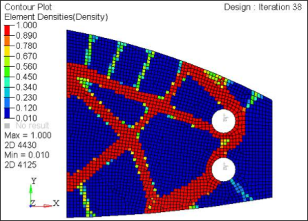
Contour of element density on the Web component from topology nonlinear gap optimization

The results from topology optimization show very discrete results as expected.

Reviewing and Comparing Results from Free-size Optimization and Topology Optimization

Results from the topology optimization show a truss type design with extensive cavities and voids, while the results from free-sizing optimization tend to come up with shear panels. While solid/void density distribution is the only choice for solid elements; for shell structures, intermediate densities can be interpreted as different thicknesses and penalizing then could result in potentially inefficient shell structures. Moreover, since a large portion of aerospace structures are shell structures, a shear panel type design is often desirable for manufacturing purposes especially for machine milled shell structures. Free-sizing optimization can prove to be very beneficial in those situations.