Model Element

Description

Param_Linear defines the solution control parameters for a linear analysis.  These parameters control the types of linear analyses to be done and the output options.

Two types of linear analyses are available in MotionSolve:

Linear analysis can be performed at any operating point.  This may be done either after a static equilibrium solution or at any point in the dynamic solution sequence.  Usually, a steady state configuration is chosen as the operating condition.  Not all the MotionSolve modeling elements are supported for a linear analysis. For more details, please see the Comments section.

Format

<Param_Linear

[    

       anim_scale              = "real"

       balancing               = {"TRUE" | "FALSE" | "AUTO"}  

       disable_damping         = {"TRUE" | "FALSE" }

       pinput_id               = "integer"

       poutput_id              = "integer"

       write_eig_info          = {"YES" | "NO"}

      write_energy_dist       = {"YES" | "NO"}

       write_matlabfiles       = {"YES" | "NO"}

       write_simulinkmdl       = {"YES" | "NO"}

       {

        ke_modes_exclude       = "string"

        ke_modes_include       = "string"

      }

       {

        se_modes_exclude       = "string"

        se_modes_include       = "string"

      }

       {

        de_modes_exclude       = "string"

        de_modes_include       = "string"

      }

  ]

/>                                                                                          

Attributes

anim_scale

Specifies a scale factor for magnifying the mode shapes during animation.

The default is anim_scale = 1.0

write_simulinkmdl

Specifies whether the A, B, C,and D matrices that are calculated are to be written out in Simulink MDL format or not.  Select from YES and NO.

The default is write_simulinkmdl = YES.

write_matlabfiles

Specifies whether the A,B,C,and D matrices that are calculated are to be written out into a file that can be read in by MATLAB.  Select from YES and NO.

The default is write_matlabfiles = YES

write_eig_info

Specifies whether the eigenvalue and eigenvector data are written to an .eig file.  Select from YES and NO.

The default is write_eig_info = YES

write_energy_dist

Specifies whether the modal kinetic strain and dissipative energy distribution is written out to the solver log file and the *_linz.mrf output file.  Select from YES and NO.  The default is write_energy_dist = NO.

See Comment 7 for more details.

pinput_id

Specifies the plant input ID used for the B and D state matrices.  Can be optionally used with the write_matlabfile and/or write_simulinkmdl option.

poutput_id

Specifies the plant output ID used for the C and D state matrices.  Can be optionally used with the write_matlabfile and/or write_simulinkmdl option.

disable_damping

Specifies whether the linearization solver should disable damping from all force elements for the eigenvalue solution.

The default is FALSE; damping will be considered for the eigenvalue solution.

ke_modes_exclude

ke_modes_include

se_modes_exclude

se_modes_include

de_modes_exclude

de_modes_include

These attributes allow you to exclude or include modes from the following energy distribution tables.

You may exclude or include modes using any one of the options below. ke_modes are used for the example, but you can use se_modes or de_modes also with these options.

ke_modes_exclude = “1”

ke_modes_include = “1”

ke_modes_exclude = “1, 2, 3”

ke_modes_include = “1, 2, 3”

ke_modes_exclude = “1:3”

ke_modes_include = “1:3”

ke_modes_exclude = “1, 2, 3:4, 5:7”

ke_modes_include = “1, 2, 3:4, 5:7”

ke_modes_exclude = “ALL”

ke_modes_include = “ALL”

ke_modes_exclude = “NONE”

ke_modes_include = “NONE”

The default for ke_modes_exclude is “NONE”

The default for ke_modes_include is “ALL”

The default for se_modes_exclude is “NONE”

The default for se_modes_include is “ALL”

The default for de_modes_exclude is “NONE”

The default for de_modes_include is “ALL”

balancing

Specifies whether the A matrix should be pre-conditioned using diagonal scaling to improve robustness of the eigenvalue solution. Choose from

TRUE: MotionSolve will always balance the A matrix using diagonal scaling

FALSE: MotionSolve will not balance the A matrix

AUTO: MotionSolve determines when to balance the A matrix based on the condition number of the eigenvector matrix. See Comment 8 for more details.

The default for balancing is AUTO

Comments

The eigenvalues and eigenvectors of a nonlinear system can change with time.  This analysis is useful for understanding the underlying vibration characteristics at a specific operating point or a series of operating points.

The eigenvalues represent the complex frequencies of vibration of the system and the eigenvectors represent the modes of vibration.

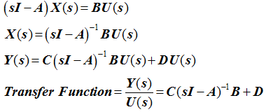
Given a set of inputs "u", a set of outputs "y" and a linearized mechanical system represented by a set of dynamical states "x", the transfer function for the system can be represented in the time domain as:

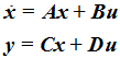
The matrices A, B, C and D are called the state matrices for the system.  If there are nx states, nu inputs and ny outputs, the dimensions of the matrices are as follows:

The inputs "u" are defined using the Control_PlantInput modeling element specified in the pinput_id and the outputs "y" are defined using Control_PlantOutput modeling element specified in the poutput_id.

State matrix output is particularly useful for control engineers, who need a linear plant representation in order to design a controller.

Another common application of state matrices is to calculate the system Frequency Response Functions to a series of time-based inputs.  This is the traditional vibration analysis of linearized mechanical systems.

Once a linear analysis is initiated, the system is linearized to the form:

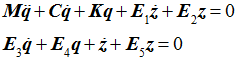
q represents the linearized displacement coordinates, z represents non-mechanical states due to other differential equations.

All constraints are eliminated from the formulation.

The equations are converted to first order form as follows:

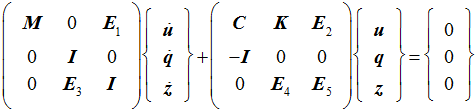
This results in the eigenvalue problem:

where

.

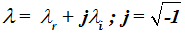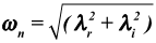
The undamped natural frequency of the this mode is:

The damping ratio for this mode is:

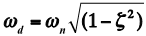
The damped natural frequency for this mode is:

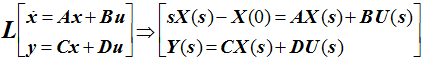
Ignoring the initial value X(0), and rearranging terms, you get:

The use of ABCD matrices to calculate the compliance transfer function about dynamic operating points overcomes all of these issues.

You may specify the modes for which MotionSolve should compute the energy distributions. This can be useful when there are a large number of modes in your system and you are interested only in the energy distribution for a subset of these modes.

You can specify the modes MotionSolve should include or exclude, separately for kinetic, strain or dissipative energy by using the following attributes:

Typically, you only need to specify the modes to be included, or the modes to be excluded, but not both. If you specify both – modes to be included and modes to be excluded, the definition that appears later in the Param_Linear statement will be honored.

Kinetic Energy:

MotionSolve computes the modal kinetic energy distribution for all bodies in the MBD model, for the modes specified. These are then written to the log file in tabular format. Each row in this table represents a body. Within a row, each number represents the percentage distribution of modal kinetic energy between the translational (X, Y, Z), rotational (RXX, RYY, RZZ) and cross-rotational, RXY, RXZ, RYZ directions of the part. The total modal kinetic energy distributions for each mode should add up to 100%.

Strain and Dissipative Energy:

MotionSolve can also compute the modal strain and dissipative energy distribution for certain force entities in the MBD model, for the modes specified (these are listed in the table below). The energy distributions are then written to the log file in tabular format. Each row in this table represents a force entity. Within a row, each number represents the percentage distribution of modal strain or dissipative energy between the translational (X, Y, Z) and rotational (RX, RY, RZ) directions.

Note: If a force entity does not contribute to the modal strain or dissipative energy, then that force entity’s row will be all zero.

In addition to the energy distribution tables, MotionSolve also displays a header for each mode that includes information about the mode number, damping ratio, undamped natural frequency and the absolute value of the modal kinetic energy. An example of this energy distribution that is written to the output log file is shown below:

*************************

Mode number           =     10

Damping ratio         =    5.0000000E-02

Undamped natural freq.=    1.5915494E+00

Kinetic energy        =    1.1427840E-05

                Percentage distribution of Kinetic energy

             |    X      Y      Z      RXX    RYY    RZZ    RXY    RXZ    RYZ

             +----------------------------------------------------------------

PART/30301   |   0.00   0.00   0.00   0.00   0.00   0.00   0.00   0.00   0.00

PART/30302   |   0.00  98.69   0.00   1.31   0.00   0.00   0.00   0.00   0.00

             +----------------------------------------------------------------

              Percentage distribution of Strain energy

             |  Total    X      Y      Z     RXX    RYY    RZZ

             +-------------------------------------------------

VFOR/30301   |   0.00   0.00   0.00   0.00

VFOR/30302   |   0.00   0.00   0.00   0.00

SPDP/303001  |   0.00   0.00   0.00   0.00   0.00   0.00   0.00

SPDP/303002  |  50.00  50.00   0.00   0.00   0.00   0.00   0.00

SPDP/303003  |  50.00  50.00   0.00   0.00   0.00   0.00   0.00

             +-------------------------------------------------

              Percentage distribution of Dissipative energy

             |  Total    X      Y      Z     RXX    RYY    RZZ

             +-------------------------------------------------

VFOR/30301   |   0.00   0.00   0.00   0.00

VFOR/30302   |   0.00   0.00   0.00   0.00

SPDP/303001  |   0.00   0.00   0.00   0.00   0.00   0.00   0.00

SPDP/303002  |  50.00  50.00   0.00   0.00   0.00   0.00   0.00

SPDP/303003  |  50.00  50.00   0.00   0.00   0.00   0.00   0.00

                 +-------------------------------------------------

These energy distributions are additionally written to the output *_linz.mrf file which may be used for post-processing.

Note: The *_linz.mrf contains information for all the modes irrespective of which were specified for inclusion or exclusion by the user.

8.

For certain models, the eigenvalues computed by MotionSolve can be extremely sensitive to small perturbations in thematrix. This occurs because the eigenvector matrix, , for such a model is highly ill conditioned. As a result, even seemingly minor changes for such models may result in large changes in the eigenvalue solution.

The condition number of a matrix, ,  is defined as

Consider the linear equation . measures the rate at which the solution will change due to a change in .

If is large, then even a small change in can cause large changes in the solution .  In such as case, the matrix is said to be ill conditioned.

To obtain a robust eigenvalue solution in such cases, MotionSolve must balance the matrix by finding a diagonal similarity transformation such that the row and column norms of are numerically close. By doing so, the eigenvector matrix becomes better conditioned and the eigenvalue solution is more robust to perturbations in .

The value of the balancing attribute controls whether matrix balancing is done or not.

•	Set this to TRUE to always balance the matrix irrespective of whether the eigenvector matrix is ill conditioned or not.

•	Set balancing to FALSE to never balance the matrix.

o	Let be the reciprocal of the condition number of

o	If , then balancing is performed

o	If , then balancing is not performed

If = 2.2E-16, then balancing is performed when R < 500 * 2.2E-16 = 1.11 E-13.

The condition number of the eigenvector matrix, , can only be computed after is computed. When balancing is set to AUTO, the eigenvalue solver may be called twice: first without balancing and then, if is small, with balancing. So an increase in run time may occasionally be seen.

Example

This example shows the Param_Linear modeling element where the energy distribution for only some of the modes is to be written out.

<PARAM_LINEAR

  ANIM_SCALE          = "1.0"

  WRITE_SIMULINKMDL   = "YES"

  WRITE_MATLABFILES   = "YES"

  WRITE_EIG_INFO      = "YES"

  WRITE_ENERGY_DIST   = "YES"

  KE_MODES_INCLUDE    = “ALL”

  SE_MODES_EXCLUDE    = “1:4, 24:36”

  DE_MODES_INCLUDE    = “1,2,3,12,13,14”

/>