Model Element
|
Description
|
Param_Static defines the solution control parameters for Static and Quasi-static analysis. These parameters control the accuracy the solution and the method to be used for solution.
MotionSolve supports two distinct methods for static analyses:
| • | A Maximum Kinetic Energy Attrition Method. |
| • | A Force Imbalance Method. |
The Maximum Kinetic Energy Attrition Method:
| 1. | The model is formulated as a dynamics problem from which all damping is removed. The result is a conservative system whose total energy, defined as the sum of kinetic and potential energies, should remain invariant with time. |
| 2. | Numerical integration is started. During integration, the kinetic energy of the system is monitored. When a peak (maximum) is detected, integration stops and backtracks as necessary to locate the peak in time, within some precision. Since the system is conservative, this instant also corresponds to a valley (minimum) for potential energy. |
| 3. | At this point, all velocities and accelerations in the model are set to zero, leading to zero kinetic energy. Then, the integration is restarted. |
| 4. | Steps 1-3 constitute one iteration. If the peak is located perfectly, then the model already is at the equilibrium configuration. However, due to the discrete nature of the integrator, this is usually not the case. Thus, it is necessary to repeat steps 1-3 until the process converges as defined by three convergence parameters: |
| • | Maximum Kinetic Energy Tolerance (max_ke_tol): This is the maximum residual kinetic of the system at the static equilibrium point. This should be a small number. |
| • | Maximum state tolerance (max_dq_tol): This specifies the upper limit for the change in system states at the static equilibrium point. |
| • | Maximum number of iterations (max_num_iter): This is the maximum number of iterations that are allowed before simulation stops. |
The Kinetic Energy Minimization method has following advantages:
| • | It only finds the stable equilibria. |
| • | It is suitable for problems where the equilibrium configuration is far from the model configuration. Such situations are problematic for the Force Imbalance Method. |
| • | It works well for contact dominated models. |
The Maximum Kinetic Energy Attrition Method has following disadvantages:
| • | It does not work with quasi-statics in the current version. |
The Force Imbalance Method:
| 1. | This method sets all the velocity and acceleration terms in the equations of motion to zero to obtain a system of nonlinear algebraic, force balance equations [ F(q, l) = 0 ]. |
| 2. | The generalized coordinates (q) and constraint forces (λ) are the unknowns. |
| 3. | The nonlinear equations are solved using the Newton-Raphson method to find the equilibrium configuration. |
| 4. | The iterations are stopped when: |
| • | The imbalance in the equations of motion is reduced below a user-specified tolerance value specified. |
| • | The equations F(q, λ) = 0 is satisfied to a user specified tolerance. |
| • | The maximum number of iterations is reached. |
The force imbalance method has the following advantages:
| • | It is a fairly reliable method and works well for a large class of problems. |
| • | It finds the solution relatively quickly. |
| • | It works for both static and quasi-static methods. |
The force imbalance method has the following disadvantages:
| • | It does not distinguish between stable, unstable, or neutral equilibrium configurations. It is equally capable of finding any of these solutions. It converges to the static solution closest to the initial configuration. |
| • | It has difficulty in cases where the equilibrium configuration is far away from the model configuration. |
| • | It has difficulty for models dominated by contact. |
The two methods, Maximum Kinetic Energy Attrition Method and Force Imbalance Method, are complementary.
|
Format
|
<Param_Static
{
[ method = "MKEAM" ]
[ max_ke_tol = "real" ]
[ max_dq_tol = "real" ]
[ max_num_iter = "integer" ] >
| [ method = { "FIM_S" | "FIM_D" } ]
[ max_imbalance = "real" ]
[ max_error = "real" ]
[ stability = "real" ]
[ max_num_iter = "integer" ]
[ compliance_delta = "real" ]
}
/>
|
Attributes
|
method
|
Specifies the choice of the algorithm to be used for Static or Quasi-static simulation. For static equilibrium, choose one of the following:
MKEAM is a method based on minimization of maximum kinetic energy.
FIM_S is a modified implementation which supports all MotionSolve elements except Force_Contact.
For Quasi-static simulation, the MKEAM method is not applicable. However, there is an additional choice called FIM_D. FIM_D is a time integration based approach to quasi-static solution. It is not applicable for a pure static solution. In addition to the parameters specified in the Param_Static element, FIM_D also uses the parameters specified in the Param_Transient element to control the DAE integration (in particular, dae_constr_tol to control the error tolerance). FIM_D defaults to FIM_S when a pure static solution is required.
In summary, both for static and quasi-static solutions, there are three choices of solvers. See Comments for their strengths and weaknesses.
The default is FIM_D.
|
max_ke_tol
|
Applicable if MKEAM was chosen. Specifies the maximum allowable residual kinetic energy of the system at the static equilibrium point. This should be a small number. The default value for max_ke_tol is 10-5 energy units.
|
max_dq_tol
|
Applicable only if MKEAM was chosen.
This specifies the upper limit for the change in system states at the static equilibrium point. The iterations are deemed to have converged when the maximum relative change in the states is smaller than this value. The default value for max_dq_tol is 10-3.
|
max_num_iter
|
Specifies the maximum number of iterations that are allowed before simulation stops. If max_ke_tol and max_dq_tol are not satisfied at this point, the equilibrium iterations should be considered as having failed. The default value for max_num_iter is 100.
|
max_imbalance
|
Applicable if force_imbalance was chosen. Specifies the maximum force imbalance in the equations of motion that is allowed at the solution point. This should be a small number. The default value for max_imbalance is 10-4 force units.
|
max_error
|
Applicable if force_imbalance was chosen. This specifies the upper limit for the change in residual of the system equations at the static equilibrium point. The iterations are deemed to have converged when the maximum residual in the equations of motion is smaller than this value. The default value for max_error is 10-4.
|
stability
|
Specifies the fraction of the mass matrix that is to be added to the Jacobian (see discussion on Newton-Raphson method in the Comments section) to ensure that it is not singular. The Jacobian matrix can become singular when the system has a neutral equilibrium solution and the initial guess is close to it. To avoid this, a fraction of the mass matrix (known to be non-singular) is added to the Jacobian in order to make it non-singular. The value of stability does not affect the accuracy of the solution, but it may slow the rate of convergence of the Newton-Raphson iterations. stability should be a small number. The default value for stability is 1e-10.
Note The square root of the value specified by stability is multiplied to the mass matrix and then added to the Jacobian to make it non-singular.
|
compliance_delta
|
Delta used during complaince matrix calculation (default = 0.001).
|
Comments
|
| 1. | For Quasi-static simulation, MKEAM is not supported. |
| 2. | While the MKEAM, FIM_D and FIM_S methods support all the following elements: |
For more details, refer to the following tables:
Table 1 - Mapping between ADAMS and MotionSolve Modeling Elements
Table 2 - Mapping between ADAMS and MotionSolve Command Elements
Table 3 - Mapping between ADAMS and MotionSolve Functions
Table 4 - Mapping between ADAMS and MotionSolve User Subroutines
MotionSolve Quasi-statics refers to the Force Imbalance method.
| 3. | The Newton-Raphson algorithm is an iterative method used to solve nonlinear algebraic equations. |
Assume, a set of equations F(Q) = 0 is to be solved. Assume also that an initial guess Q* is available.
Let Q be partitioned into two sets of coordinates Qt, Qr, where Qt are the translational coordinates, and Qr the rotational coordinates:
QT = [ QtT, QrT ].
Let NORM(x) be a function that returns the infinity norm of any array x. In other words, the maximum of the absolute value of the components of x.
If NORM(F(Q*)) < max_imbalance, Q = Q* is the solution. However, this does not always happen. It is much more common to find that NORM(F(Q*)) >> max_imbalance.
The Newton-Raphson method is an iterative process for refining the initial guess Q* so that the equations F(Q) = 0 is satisfied. The algorithm proceeds as follows:
| 1. | Set iteration counter j = 0. Set Qj = Q*. |
| 3. | If NORM (F(Qj)) < max_imbalance, skip to step 10. |
| 4. | Evaluate Jacobian, J = [ Fi/Qj]. Fi/Qj]. |
| 5. | Calculate ΔQj by solving the linear equation J*ΔQj = -F(Qj). |
| 8. | If j < max_num_iter, go to step 2. |
| 9. | Else: iterations did not converge to a solution; exit. |
| 10. | Iterations converged; exit. |
| 4. | Finding the static equilibrium configuration for nonlinear, non-smooth systems is difficult. You may find that the default parameters do not work very well for all models. Here are some tips for obtaining successful static solutions using "The Force Imbalance Method": |
| • | Make sure that your system starts in a configuration close to a static equilibrium position. |
| • | Look at the animation of the static equilibrium iterations to understand what the algorithm is trying to do. Visual inspection is crucial for gaining an insight into the behavior of the algorithm. |
| • | Sometimes, it is useful to have several static iterations to obtain the final solution. Here is how the outer iterations could work: |
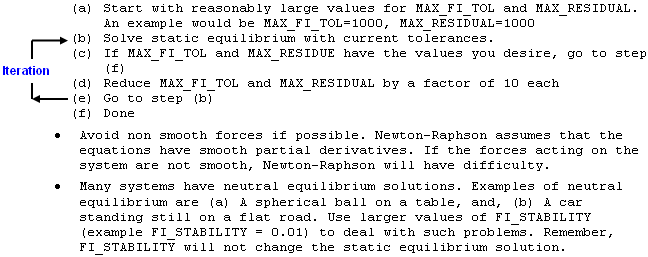
| 5. | Avoid non smooth forces if possible. Newton-Raphson assumes that the equations have smooth partial derivatives. If the forces acting on the system are not smooth, Newton-Raphson will have difficulty. |
| 6. | Many systems have neutral equilibrium solutions. Examples of neutral equilibrium are (a) a spherical ball on a table, and, (b) a car standing still on a flat road. Use larger values of stability (example stability = 0.01) to deal with such problems. Remember, stability does not change the static equilibrium solution. |
| 7. | When used for quasi-static, FIM_S involves a sequence of static simulations. In contrast, FIM_D method uses the DAE integrator DASPK to perform quasi-static simulation. Hence, FIM_D uses the DSTIFF parameters specified in the Param_Transient element to control the integration process (in particular, dae_constr_tol to set the error tolerance), in addition to the parameters specified in the Param_Static element. FIM_D always uses I3 DAE formulation. |
| 8. | FIM_D uses FIM_S at the start and the end of the quasi-static solution. FIM_S is also used when the integrator encounters difficulties. Thus, the error tolerance setting for FIM_D is Param_transient::dae_constr_tol except for the first and last steps, which use the error tolerances in Param_Static for FIM_S. |
| 9. | FIM_D is usually much faster than FIM_S for quasi-static simulation. |
|
Example
|
This example shows the default settings for the Param_Static element that uses the MKEAM method.
<Param_Static
method = "MKEAM"
max_ke_tol = "1.000E-05"
max_dq_tol = "0.001"
max_num_iter = "100"
/>
This example shows the default settings for the Param_Static element that uses the FIM_S solution method.
<Param_Static
method = "FIM_S"
max_residual = "1.000E-04"
max_imbalance = "1.000E-04"
max_num_iter = "50"
/>
|


